AI Architect - Advanced deep learning settings
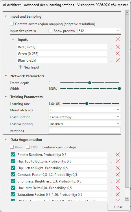
The AI Architect allows the user to control deep learning settings with respect to Input and Sampling, Context-aware region mapping, Network Parameters, Training Parameters, and Data Augmentation.
The AI Architect is opened by pressing the Advanced Deep Learning settings button  under Classification.
Input and Sampling
Context-aware region mapping
Context Aware Region Mapping is a special tool for anatomical region segmentation (e.g. brain and spinal cords regions, kidney regions etc.), where tissue contrasts are not always sufficient for accurate segmentation and contextual information of the entire tissue section is needed. It can be useful for segmentation tasks where the regions differ in size or shape from tissue to tissue due to its adaptive resolution capabilities, e.g. different sections throughout the brain volume.
Activating Context Aware Region Mapping will change the sampling strategy to ROI(s) instead of labels during training of the deep learning network. That means, magnification (which is normally fixed), becomes adaptive and selects the optimal magnification for each specified ROI. Context Aware Region Mapping therefore enables multiple regions trained at multiple resolutions (adaptive resolution).
Context Aware Region Mapping can be activated for all Deep Learning classifiers. However, DeepLabv3+ is generally recommended due to its global context capabilities. Because the ROI now serves as sampling object, make sure to include an ROI that outline the tissue section and covers all annotated labels (the ROI would normally be the outline of your tissue).
Example Workflow
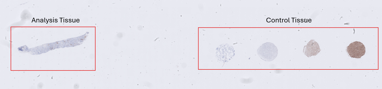
An alternative application of Context Aware Region Mapping is in control studies where both analysis tissue and control tissue are present on the same slide. In such setups, the analysis tissue is often located in one region of the slide, while control tissue is placed elsewhere for reference or validation purposes. For downstream quantitative analysis (e.g. object counts, size measurements, or other metrics), it is essential that a classification APP is restricted to classify only the analysis tissue as tissue, as inclusion of control tissue would lead to misleading results.
Standard deep learning APPs can struggle in this scenario, as control tissue often exhibit visual characteristics similar to those of the analysis tissue. As a result, standard APPs often incorrectly segment both regions as tissue. Context Aware Region Mapping addresses this challenge by incorporating global contextual information from the entire slide, enabling the APP to distinguish between analysis tissue and control tissue based not only on appearance but also on spatial context.
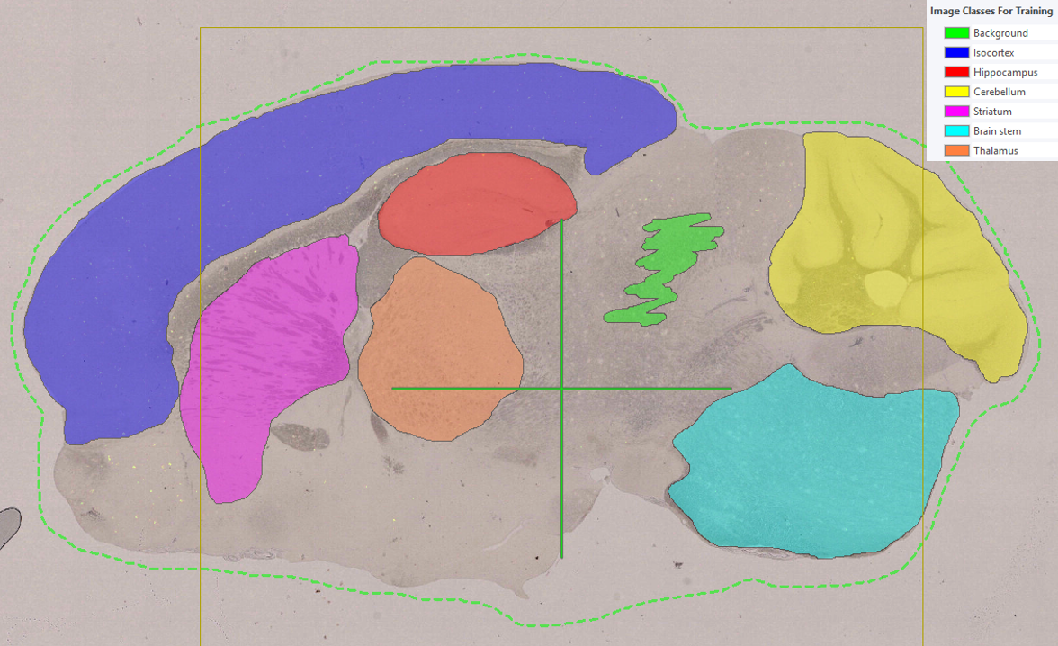
Below, a step-by-step example illustrates how Context Aware Region Mapping can be used to solve this problem. The objective in this example is to classify solely the analysis tissue in the following image as tissue.
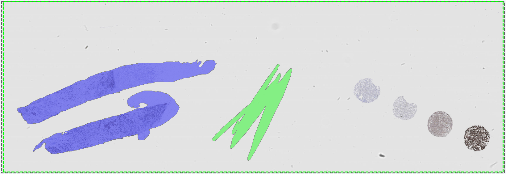
To avoid overfitting, the APP is trained on a different image that, like the target image, contains both analysis tissue and control tissue. Training labels are drawn in the standard manner, with analysis tissue labeled as tissue and including an example of background. The standard workflow is described in Getting Started.
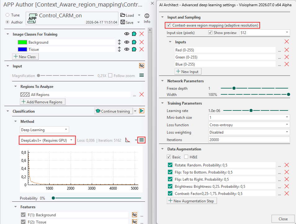
The APP is then configured as follows: Context Aware Region Mapping is enabled in the Advanced Deep Learning settings ![]() by toggling on Context Aware Region Mapping (Adaptive Resolution). The Deep Learning model DeepLab3+ is selected, and the APP is otherwise configured according to the standard setup procedure before training is started. As Context Aware Region Mapping selects the optimal magnification for each specified ROI, the Magnification setting under Input is disabled. In this example, the APP is trained for 5,162 iterations, at which point the loss curve has plateaued. For larger studies with more extensive training datasets, additional training iterations may be required.
by toggling on Context Aware Region Mapping (Adaptive Resolution). The Deep Learning model DeepLab3+ is selected, and the APP is otherwise configured according to the standard setup procedure before training is started. As Context Aware Region Mapping selects the optimal magnification for each specified ROI, the Magnification setting under Input is disabled. In this example, the APP is trained for 5,162 iterations, at which point the loss curve has plateaued. For larger studies with more extensive training datasets, additional training iterations may be required.
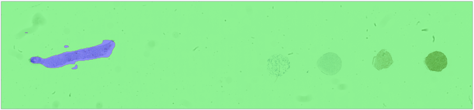
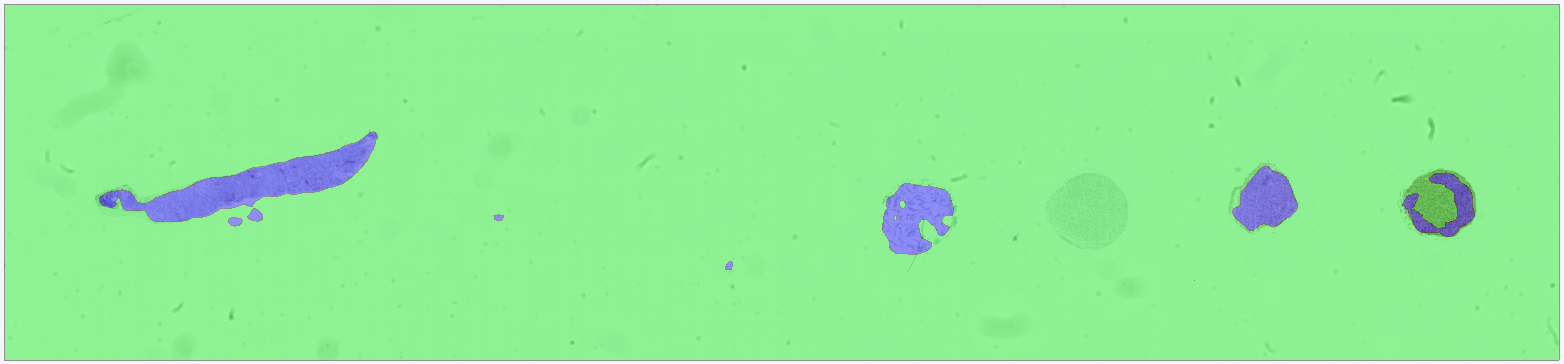
After training, the APP is run on the target image. The results show that the APP successfully differentiates between analysis tissue and control tissue, such that only the analysis tissue is classified as tissue.
For comparison, a second APP is trained under identical conditions (same training data, same model architecture, and the same number of training iterations) but without Context Aware Region Mapping enabled. In this case, the APP incorrectly classifies the control tissue as tissue, demonstrating the limitation of standard deep learning approaches when contextual information is not considered.
- Because the resolution is adaptive, make sure to checkmark Treat Regions Individually in the Advanced Setup under Input, when running the APP in images with multiple tissue sections (ROIs). Otherwise the FOV
can expand to fit all ROIs within one FOV, i.e. the samples are not analyzed one by one.
- If you switch Deep Learning classifier, make sure to re-activate Context-Aware Region Mapping in the AI architect.
- Make sure to include an ROI that outline each tissue section. The ROI should outline the relevant tissue with the context needed to segment the areas of interest.
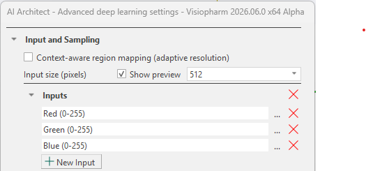
Input Size (Pixels)
The input size is used to control the size (width and height in pixels) of each image patch sent through the network. This parameter determines the network's effective receptive field, i.e., the amount of surrounding tissue context available during training. The receptive field can be adjusted through the magnification and/or the input size. Generally, problems that depend primarily on local information (e.g., nuclei or membrane segmentation) typically require smaller input sizes, since only the immediate neighborhood contributes meaningfully to the classification. On the other hand, larger structures (e.g., metastases or vessels) benefit from a broader contextual view. To accommodate such structures, a larger receptive field is required, which can be achieved by increasing the input size and/or reducing the magnification so that a larger region of tissue is represented in each patch.
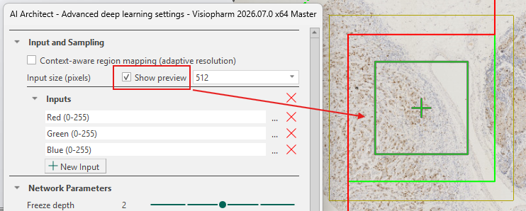
Larger input sizes result in slower training due to longer iteration times, while smaller input sizes allow faster iterations. However, the input size must be sufficiently large to fully capture the target structure to ensure effective training. The input size can be viewed by toggling the Show preview check-box, as shown below. The green box with a cross in the middle indicates the size of a single input patch sent through the network using the current input size.
After training, the input size cannot be changed unless the trained network is discarded.
The input size of a neural network and the APPs' FOV Size are not the same. The FOV size is part of the APP's overall image-processing pipeline. The input size is used solely during the deep learning model's patch extraction.
Inputs
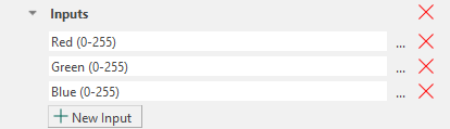
The Inputs section defines the image channels provided to the neural network. Networks can be configured for brightfield, fluorescence, or IMC images, including cases where aligned WSS channels are available. When multiple aligned modalities exist, they can be combined as cross-channel inputs and processed jointly by the network.
When working on brightfield images (which contain RGB bands), the default inputs will be the Red, Green, and Blue bands. When working on fluorescence images, the default inputs will be all available color bands, and it is therefore necessary to manually adjust this to a maximum of three inputs. Manual adjustment also applies to IMC images and multiple aligned modalities. It is therefore recommended to always ensure that the network takes a maximum of three inputs, as the default can exceed three and thereby hinder training. An explanation for this behavior is detailed below.
Any selected band can be removed by clicking the ![]() icon. It is also possible to adjust the Min and Max values by clicking the
icon. It is also possible to adjust the Min and Max values by clicking the ![]() icon.
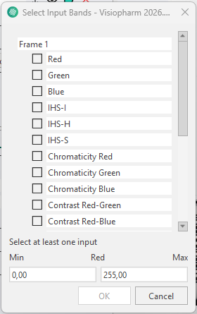
The Min and Max can also be set when creating a new input band, at the bottom of the Select Input Bands tab.
icon.
The Min and Max can also be set when creating a new input band, at the bottom of the Select Input Bands tab.
New input bands can be added by clicking the ![]() button. This opens the Select Input Bands tab, where any available band from the loaded image channels can be enabled as an input to the neural network. It is possible to select a wide variety of inputs, ranging from RGB color bands to deconvolutions and even features.
button. This opens the Select Input Bands tab, where any available band from the loaded image channels can be enabled as an input to the neural network. It is possible to select a wide variety of inputs, ranging from RGB color bands to deconvolutions and even features.
More information about the available bands can be found in the Bands section.
Selecting the number of input bands
When a new APP is created with three or fewer input bands, the first layers of the neural network (the encoder) are initialized using a set of parameter weights taken from a pretrained model developed by Visiopharm. This pretrained model was trained on data with exactly three input bands, and its weights provide a stable starting point that generally requires fewer annotations and can reduce the risk of overfitting.
If a single input band is selected, it is internally duplicated to create three inputs. If two input bands are selected, a third band is generated as the mean of the first two. These adjustments allow the pretrained weights to be applied correctly.
When more than three input bands are selected, pretrained initialization cannot be applied. In this configuration, all network weights are initialized randomly, which increases the amount of annotated data required and necessitates longer training to achieve stable performance.
Selecting more than 3 input bands is not advised, as it prevents the network from being initialized with pretrained weights and therefore significantly hinders training.
Multiselecting bands for an input
Certain analysis workflows, such as cell detection across multiple biomarkers, may require information from several independent bands. Many immunofluorescence markers (e.g., CD45, CD56, CD68, DAPI, CD11b, CD20, Vimentin, Na/K ATPase) highlight distinct cell populations, and combining several of these markers can improve detection performance. To support such use cases while maintaining compatibility with pretrained initialization, multiple bands can be merged into a single input. This is done directly in the Select Input Bands dialog by selecting multiple bands simultaneously. The selected bands are then combined into a single composite input (e.g., CD45 + CD56) that is treated as one input band by the neural network.
Once the training is complete, removing or adding an input will delete any training done by the APP and require the APP to be retrained. It is possible to replace an input with another; however, depending on the data, additional training after replacement might be needed.
Preprocessing of inputs
All selected input bands undergo automatic preprocessing to stabilize and improve network training. For RGB-based inputs, the bands are standardized by subtracting a mean value from each band. For non-RGB inputs (e.g., fluorescence or IMC), each band is normalized using an estimated minimum and maximum value so that all inputs operate on a comparable scale. These preprocessing steps are applied automatically.
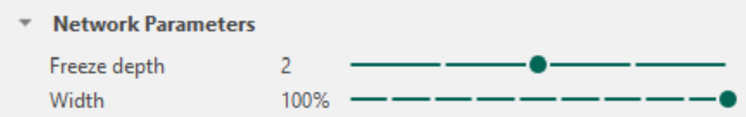
Network Parameters
In the Network Parameters section it is possible to reconfigure elements of the selected network architecture. Specifically, a Freeze Depth and a Width percentage can be defined. Adjusting these parameters can improve training stability for sparse datasets that are prone to overfitting, or increase efficiency when training on very large datasets.
To understand the effect of these settings, it is helpful to recall the structure of the selected architecture. A description of each architecture is provided under Network Architecture.
Freeze depth
The depth of a neural network corresponds to the number of encoder blocks used to downscale the input image and extract features. For example, the U-Net encoder contains four blocks. For networks trained with three or fewer input channels, each of these blocks is initialized with filters with pretrained weights. These pretrained filters extract general low-level features such as edges, curves, and simple textures. During training, these weights are updated to specialize the feature extraction for the specific classification task.
When the training set is sparse, meaning it contains few annotations or limited variation, the risk of overfitting increases. In such cases, updating all pretrained filters may cause early layers to adapt too strongly to dataset-specific artifacts, thereby reducing generalization on new images and ultimately leading to poorer predictions on images the APP has not been trained on. Adjusting Freeze Depth prevents this by keeping early encoder blocks fixed so that the weights in these blocks are not updated during training.
For example, a freeze depth of 1 preserves all pretrained weights in the first encoder block, while deeper blocks remain trainable. A higher freeze depth value freezes additional blocks. For large and diverse datasets with low overfitting risk, freezing blocks is generally unnecessary. The default setting is Freeze Depth = 0, meaning all encoder blocks are trainable.
Freeze Depth When Continuing Training
When continuing training on an existing network, all weights are initialized from the previously trained state. The appropriate freeze depth depends on how much the new dataset deviates from the original dataset used to train the APP.
-
Minor variation (e.g., new staining variation within the same tissue type): Such changes primarily influence the deeper encoder blocks, where task-specific and high-level features are represented. In these cases, the low-level features in the early blocks remain valid, and fine-tuning only the deeper blocks is sufficient. A higher freeze depth can therefore be used, keeping the early blocks fixed while allowing the deeper blocks to adapt to the new data.
-
Substantial structural differences (e.g., features or patterns not present in the original dataset): Such differences influence both low-level and high-level feature extraction. The early encoder blocks must therefore be retrained to learn new structural information. This requires a lower freeze depth (for large changes often 0), ensuring that more blocks remain trainable.
Be aware that when continuing training with new data, the learning rate should also be adjusted, as freeze depth does not control how strongly the updated layers adapt to the new data.
Width
The Width parameter defines the percentage of filters retained in each convolutional layer relative to the default architecture.
A width of 100% preserves the full original network size.
Reducing width creates a smaller network with fewer parameters, leading to faster training, but also reducing the network's ability to capture complex patterns.
A network that is too wide may overfit, as the high complexity of the model allows it to learn patterns that carry no meaningful information or to focus on dataset-specific artefacts rather than learning to generalize relevant biological structures.
In contrast, a network that is too narrow (a low width percentage) may lack sufficient capacity for difficult classification tasks. For example, a very low width may prevent the network from distinguishing subtle structural differences between similar tissue types.
As a rule of thumb, a width of 100% is typically required for complex classification tasks, whereas a lower width percentage can be beneficial in cases where training is slow (e.g. due to a very large dataset), and the classification task is relatively simple.
Adjusting width therefore provides a practical way to balance generalization, training speed, and model complexity.
When width is set below 100%, only a random subset of pretrained filters is used for initialization. This yields partially pretrained weights and typically requires that all layers remain trainable.
When using a width below 100%, it is recommended to set freeze depth to zero to ensure effective adaptation to the reduced architecture.
Changing the width after training removes the existing training results because a new network must be constructed based on the updated settings.
Training Parameters
Training refers to the repeated process in which the network analyzes image patches, produces a classification, and gradually updates its weight parameters based on how well the predictions match the provided labels or annotations.
The training process is monitored using a loss function, which can be viewed by clicking the  icon in the App Author Classification section. The loss plot shows the loss value as a function of training iterations; lower loss values indicate better predictive performance.
Training is generally continued until the loss curve stabilizes at a low value, indicating convergence. Adjusting the training parameters can help achieve convergence more efficiently, improve training stability, and reduce loss fluctuations, thereby shortening training time and helping reach reliable results more quickly.
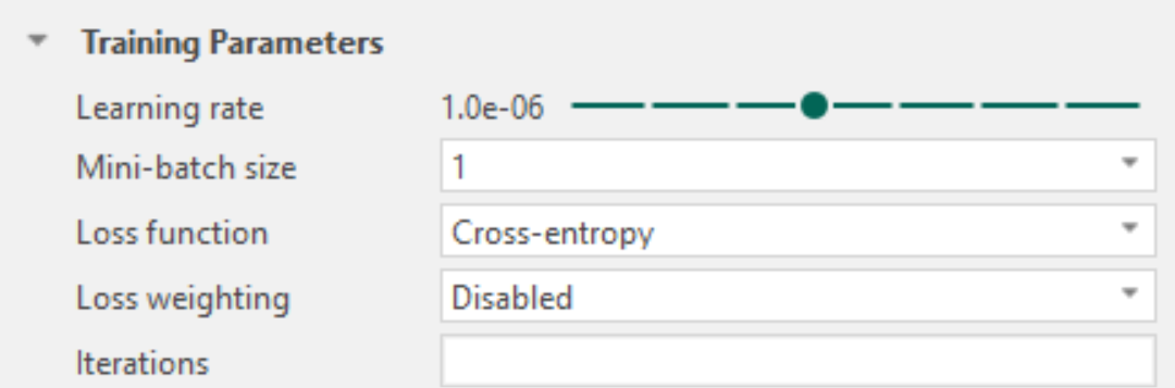
Learning rate
During each training iteration, the network produces a classification and updates its weight parameters based on how well the predictions match the provided labels or annotations. The learning rate controls the size of these parameter updates and therefore determines how quickly and how stably the network learns.
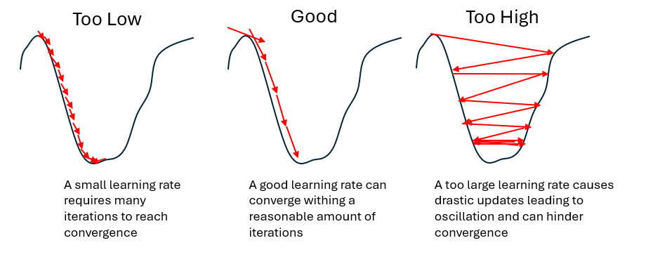
A low learning rate results in small, cautious updates of the weight parameters. This leads to stable training behavior and precise refinement, but typically requires many iterations before the loss stabilizes at a low value. Low learning rates are particularly suitable for fine-tuning an already trained model with new data or for late training stages where only small improvements are desired.
A high learning rate allows larger changes to the weight parameters between iterations. This can speed up training, especially in early stages, but increases the risk of instability. If the learning rate is too high, the training process may overshoot good solutions, leading to strong fluctuations or increases in the loss curve.
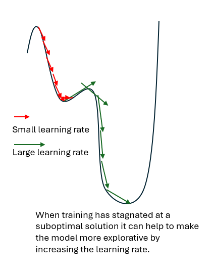
In some cases, training may stabilize at a local minimum, meaning a solution that is better than nearby alternatives but not the best possible (global) solution. If this local minimum is shallow or suboptimal, the network may fail to capture important structures in the data. Increasing the learning rate can help the training process move out of such regions which may lead to better overall performance.
Selecting an appropriate learning rate is therefore a balance between training speed, stability, and the ability to reach a good solution, (e.g., produce satisfactory predictions ).
The learning rate should be lowered when:
- The loss curve fluctuates strongly or increases, indicating unstable training.
- Training has reached a stable phase and further refinement is desired.
- Fine‑tuning a pretrained model to adapt it to new data or labels/annotations.
The learning rate should be increased when:
- The loss curve decreases steadily but very slowly.
- Early training progresses slowly despite stable behavior.
- Training appears to have converged to a shallow or suboptimal local minimum, and relevant structures are not adequately captured.
As a rule of thumb:
- Increase the learning rate when the goal is faster progress or broader exploration, particularly in early or stalled training.
- Decrease the learning rate when the goal is stable refinement, particularly in late training or fine-tuning.
Selecting an optimal learning rate is largely empirical. The default learning rate is suitable for most use cases and should be used as a starting point. Early training often exhibits loss fluctuations and this is not necessarily problematic. Learning rate settings should be evaluated based on overall loss behavior across multiple iterations (e.g. strong fluctuations, divergence, or very slow improvement).
Mini-batch size
During training, the dataset is processed in smaller subsets called mini-batches. For each mini-batch, the network produces predictions and updates its weight parameters based on the combined result of all samples in that batch. The mini-batch size determines how many image patches contribute to a single weight update.
The default mini-batch size of 1 means that the network updates its parameters after each individual image patch. This allows frequent updates but can result in unstable training behavior, as consecutive image patches may differ substantially. Larger mini-batch sizes combine information from multiple image patches before updating the network parameters. This averaging effect leads to smoother and more stable training behavior, as individual variations have less influence on each update.
Increasing the mini-batch size generally improves training stability but requires more GPU memory. Systems with limited hardware resources may therefore require smaller mini-batch sizes.
When increasing the mini-batch size, it is often possible to also increase the learning rate, as the smoother updates allow larger parameter changes without destabilizing training.
Loss function
The loss function defines how the network evaluates the quality of its predictions during training. It provides a numerical measure of the difference between the predicted classification and the provided labels or annotations. Training aims to minimize this value; lower loss indicates better agreement between prediction and annotation.
Different loss functions emphasize different aspects of classification quality. Selecting an appropriate loss function should therefore be based on the characteristics of the data and the classification task.
Visiopharm supports the following loss functions:
Cross-entropy, Intersection-over-Union (IoU), and IoU + Cross-entropy.
Cross-entropy evaluates classification accuracy on a pixel-by-pixel basis by comparing the predicted class of each pixel with the corresponding label or annotation. It is the most commonly used loss function and the default choice in Visiopharm. Cross-entropy is suitable for the majority of classification tasks and is particularly useful when large regions of the data consist only of background and no foreground classes.
A use case where Intersection-over-Union (IoU) can be advantageous is when foreground classes occupy a very small fraction of the image compared to the background. In such cases, cross-entropy may favor correct background classification at the expense of foreground detection. For example, if only 5% of pixels represent tumor tissue and the remaining pixels represent stroma, a model that classifies all pixels as stroma would achieve high pixel-wise accuracy but produce a practically useless result. IoU evaluates how well the predicted foreground regions align with the annotated foreground regions. Correctly classifying background pixels does not improve the IoU score, while missing or incorrectly predicting foreground regions leads to a high loss. IoU can therefore encourage accurate detection of small foreground structures. However, IoU is only appropriate when foreground pixels are present in every, or almost every, training region.
As an alternative to changing the loss function, class imbalance can also be addressed by applying loss weighting when using cross-entropy.
IoU + Cross-entropy combines pixel-wise classification accuracy (cross-entropy) with region-level alignment (IoU), balancing local accuracy with overall classification quality. This loss has shown good performance for tasks with varying class sizes, such as brain region classification, particularly when Context Aware-Region Mapping is enabled.
Loss weighting
Loss weighting is applicable only when using cross-entropy. It allows selected classes to contribute more strongly to the loss during training and should be used with caution. Extreme weight values can lead to unstable training. Loss weighting is primarily used to address class imbalance, where some classes are underrepresented relative to others. In such cases, the network may otherwise prioritize correct classification of dominant classes while neglecting smaller or less frequent classes. By increasing the contribution of underrepresented classes, loss weighting enables cross-entropy to remain effective even when foreground classes occupy only a small fraction of the data.
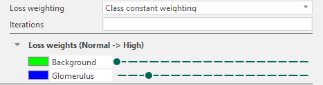
In Visiopharm, loss weighting is enabled by changing the Loss weighting setting from Default to Class constant weighting. Once enabled, a list of classes defined in the APP is displayed, each associated with a weight level ranging from Normal to High.
The leftmost position corresponds to equal weighting across all classes. Moving the slider to the right increases the weight of the corresponding class, meaning that misclassification of this class contributes more strongly to the loss during training.
Iterations
The Iterations parameter defines the maximum number of training iterations performed before training stops automatically.
Leaving this field blank disables automatic stopping, allowing training to continue until manually stopped. The field is blank by default.
When continuing training on an already trained network, defining iterations will specify the number of additional iterations. (For example, if a network is trained for 500 iterations and iterations is set to 550 when continuing training, this will result in the training stopping after 1,050 iterations.)
Data Augmentation
Data augmentation is a technique used to artificially increase the size and diversity of a training dataset by applying controlled transformations to the existing data. This approach is particularly useful when the available dataset is small, as is often the case in medical studies, and helps deep learning models generalize better to unseen data by exposing them to a broader range of variability. Data augmentation applies image transformations to the receptive field fed into the network during training, while preserving the underlying labels or annotations.
For example, in a small dataset, tissue samples may consistently be placed on the glass slide with a similar orientation. This can unintentionally cause the model to learn orientation-specific features, such as assuming that a structure of interest is always elongated in a particular direction. By applying spatial transformations such as rotation, the orientation of the tissue is varied, reducing this bias and making the model more robust to differently oriented samples.
Augmentation Types
Augmentation types are grouped according to whether they affect color, spatial orientation, or stain appearance. These augmentations introduce color, spatial, and stain variability, encouraging the model to become invariant to these factors.
Color: Contrast, Brightness, Hue, Saturation
Spatial: Rotate, Flip
Stain: H&E, HDAB
Contrast
Contrast changes the contrast of each input image with a random factor in a user-defined range with a selected probability
where is the random factor and and are the lower and upper range values.
Brightness
Brightness changes the brightness of each input randomly by a user-defined factor with the selected probability
where is the user defined factor, and is the selected brightness value, and is the estimated maximum value of the input.
Hue
Hue changes the hue of the color in each input randomly between a user-defined factor with the selected probability. Initially, it involves the transformation from RGB-space to IHS-space followed by a perturbation of .
where is the random factor, and is the selected hue value.
Saturation
Saturation changes the saturation of the color in each input in a user-defined range with a selected probability. Initially, it involves the transformation from RGB-space to IHS-space followed by a perturbation of .
where is the random factor, and a and b are the lower and upper range values.
Rotate
Rotation augments the original image by a certain spatial rotation. This aims to make the network invariant to rotations, which is usually the case in histopathology (the tissue can be put in many ways onto the glass slide).
All transformations should be valid when analyzing anatomical sections.
Flip
Flip is a popular augmentation technique that allows for horizontal and vertical invariance. As for rotation, this is usually a valid transformation in histopathology. This step can be added as Left to Right or Top to Bottom.
H&E staining
This step uses a domain‑specific data augmentation approach that augments H&E stain intensities by randomly varying fixed H&E stain vectors. Rather than applying arbitrary color perturbations, the augmentation targets variability that is well defined by the H&E dyes.
In digital histopathology, fixed stain vectors can be defined for hematoxylin and eosin, which are leveraged in this approach. A color deconvolution method based on an optical density (OD) transform is used to project the image onto the H and E stain vectors.The degree of augmentation can be adjusted independently for each stain, allowing greater variation to be introduced for stains that exhibit higher variability in the data, such as eosin relative to hematoxylin.
HDAB staining
Augmentation Configuration
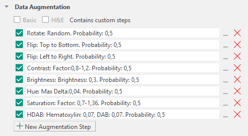
Visiopharm applies a predefined set of data augmentation steps by default. Each augmentation step can be removed using the ![]() icon or reconfigured using the
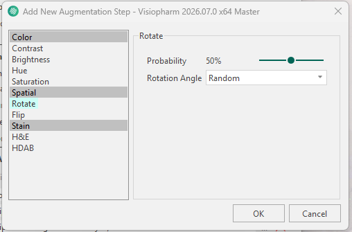
icon or reconfigured using the ![]() icon. The available configuration options depend on the selected augmentation type (for example, rotation can be configured as random or fixed-angle rotation, and brightness can be adjusted to a specified intensity range).
icon. The available configuration options depend on the selected augmentation type (for example, rotation can be configured as random or fixed-angle rotation, and brightness can be adjusted to a specified intensity range).
Augmentations in Visiopharm are applied sequentially as a pipeline. Each augmentation step is evaluated independently for every receptive field processed during training.
Each augmentation step has an associated probability parameter that determines how often the transformation is applied to a receptive field. By default, this probability is set to 0.5 and can be adjusted individually for each augmentation type.
Additional augmentation steps can be added using the  icon, which opens the New Augmentation Step menu where an augmentation type can be selected and configured.