Using Deep Learning in Visiopharm

This section provides a guide to creating a deep learning app in Visiopharm. It includes a step-by-step walkthrough of both the setup and training process, supplemented with further details on how to configure and understand the training process, the loss curve and the feature generation. In addition, common errors are highlighted, with guidance on how to avoid them. The section lastly introduces the use of TensorBoard as a tool for gaining deeper insight into the training process.

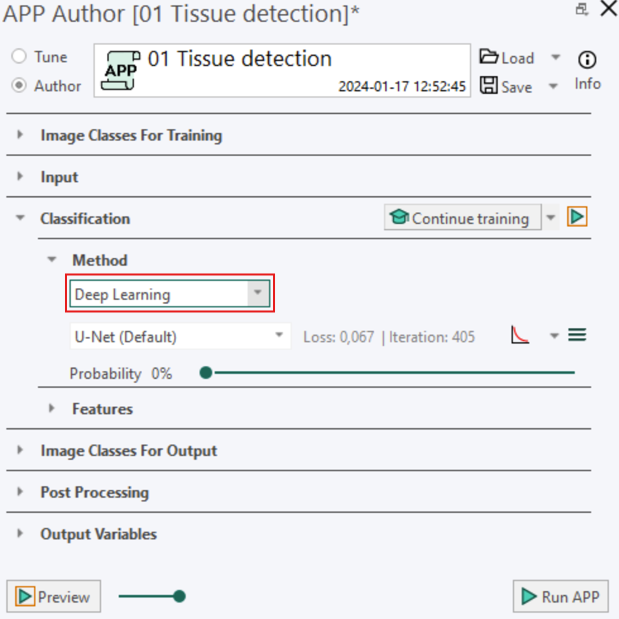
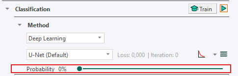
The deep learning method is accessed through the Classification section in the App Author dialog, as illustrated below.

The Deep learning Method in the Classification section of the APP author.

Creating a Deep Learning APP - Step by Step Guide

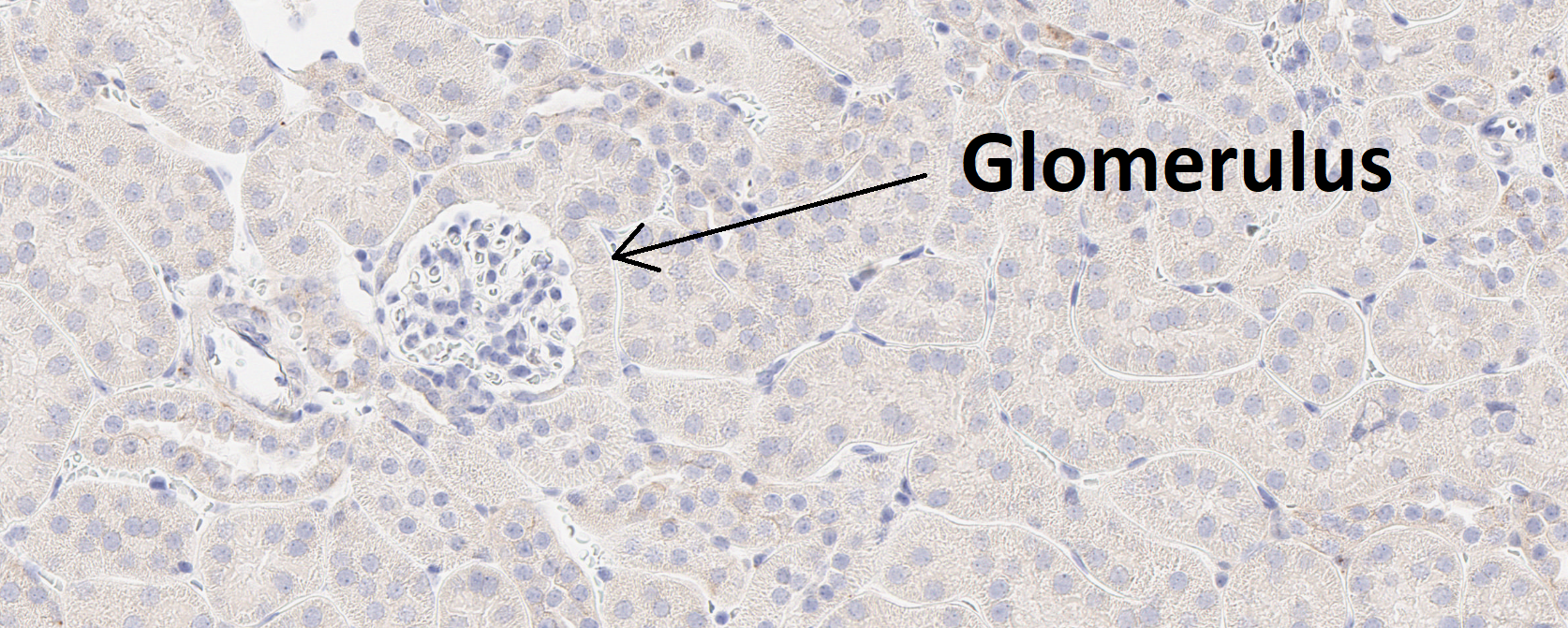
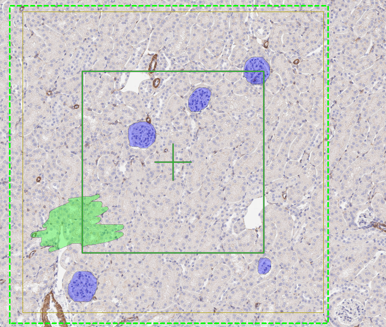
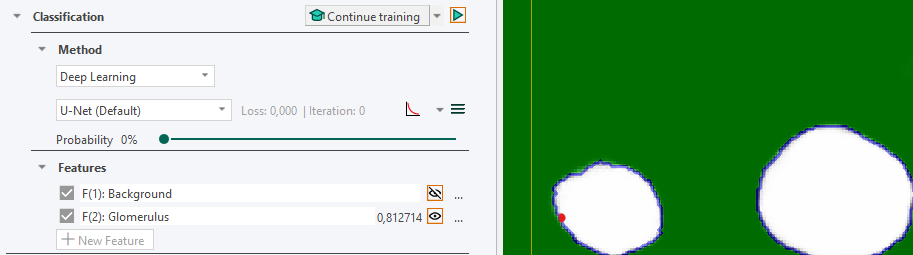
This guide provides a simple entry point for creating a deep learning app. The goal is to build an APP that can automatically detect glomeruli, which are small structures in the kidney, as shown in the image below.

Image illustrating the example task: detecting glomeruli in kidney tissue (Kidney CD68)

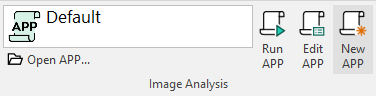
1. Create a new APP by pressing the New APP button in the Image Analysis section in the ribbon.

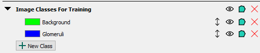
2. Create an image class in the Image Classes for Training section for each image structure of interest, as well as a background class. When using ROIs for training, the background class must be placed at the top of the image class list. In this example, we aim to detect a single image structure, glomeruli, and therefore define two image classes in total, including the background class.

3. Draw training labels on all instances of the image structure of interest (in this case, glomeruli) across the entire training slide(s). This requires that every glomerulus is labeled, and that at least one example of the background class is included. If Regions of Interest (ROIs) are drawn on the slide, all pixels within each ROI will be used for training. Pixels inside an ROI that are not explicitly labeled are assumed to belong to the first training label, which in this case is Background. To guide the sampling process correctly, at least one explicit example of the background class must be provided by drawing a background training label.

Example of drawn labels on the glomeruli structures (blue), one exemplary background label (green) and a square ROI (green).

In some cases, such as tumour-stroma classification, a background class may not be meaningful. In these situations, it is recommended that the first class in the image class list represents the largest class, which is often stroma. This approach is generally easier, as it requires labeling instances of tumour and providing at least one example of stroma. All unlabeled pixels will then be automatically classified as stroma.

When drawing ROIs around training labels, keep the following guiding principles in mind:

• Drawing ROIs that are too small can reduce the dataset size and cause the model to overfit, leading to incorrect predictions.
• Avoid drawing ROIs that cut through an object, as this teaches the algorithm that the object should be split.
• Do not draw labels outside ROIs, as this can interfere with the training process.
• If possible, square ROIs often result in more effective training; however, any ROI shape that follows the above principles works.

If ROIs are not drawn on the slide, only pixels with training labels are used for training. This approach can be useful when it is not feasible to label all objects of interest, and you want to avoid automatically classifying all unlabeled pixels as background. In such cases, some unlabeled pixels may still belong to the object of interest but remain intentionally unclassified.

4. Set up the Input section with the desired magnification. A high magnification means that fine details in the image are visible to the app, while a low magnification means that only large-scale details are visible. To see the magnification click on the icon. The lower the magnification, the faster the training. Therefore, the magnification level should be chosen as low as possible while ensuring that the objects of interest are still visible.

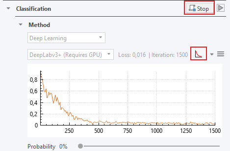
5. Under the Classification -> Method, select Deep Learning as the classifier. Leave the settings at the default settings (U-Net (Default), Probability= 0%)

6. Press the train button to start training the APP. After a short delay, the loss curve shown to the right of the network architecture name will fluctuate and decrease.

7. While the APP is training, you can click on the training plot icon if the convergence graph is not visualized. When the training seems to have converged, you can stop the training by clicking the stop button .

Training example over 1500 iterations. During the initial phase, the loss decreases, indicating that additional training improves model performance. After approximately 500 iterations, the loss stabilizes, suggesting convergence and that further training is unlikely to improve the APP. Note that more than 1500 iterations is often required in practice.

8. Save the APP together with the trained neural network by pressing the save button , at the top of the APP Author dialog.

9. Preview. Previewing the APP classifies the current field of view (FOV). Click the Preview button under Classification to view and assess the neural network output.

Example: Previewing the result of a Glomeruli detection APPs

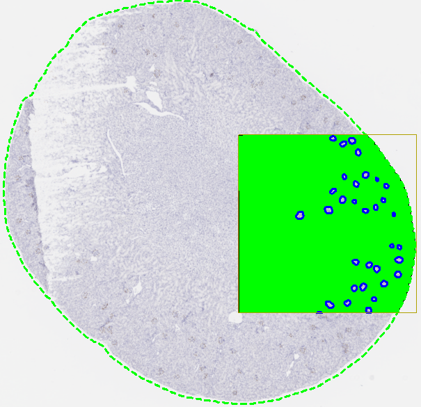
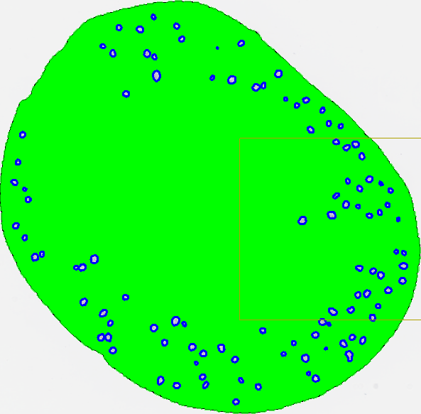
10. Run the APP. When training is satisfactory (i.e., the preview looks good) run the APP to classify the entire slide by clicking .

Example: Running a Glomeruli detection APP

tip

After training, classification results will often still contain minor misclassifications or require refinement. While post-processing is not strictly required, it is commonly used in full analysis workflows to improve results. Typical post-processing operations include morphological steps such as erosion, dilation, and hole filling. Post-processing steps can also be used to adapt the output for further analysis, for example by converting classified objects into ROIs or clearing the background label. For details on available post-processing operations, see the Post Processing section.

For information on creating output variables for further analysis (e.g. counting classified glomeruli), see the Output Variables section.

Training a Deep learning APP

Training is the defining component of deep learning and forms the foundation of how a deep learning model is built. For an overview of how training fits into the overall deep learning pipeline, see the Basic Deep Learning Pipeline Section. This section builds on the step-by-step guide by expanding on the training steps, providing additional background, practical considerations, and guidance to help ensure successful training.

Before starting the training process of the classifier, ensure that the following conditions are met:

• Each type of object you want to detect in the image has a corresponding image class defined in the Image Classes for Training section of the APP Author.
• Each training slide or image contains one or more training ROIs, and no labels are drawn outside of these ROIs.
• Every object of interest present within the training ROI(s) is labeled with its corresponding image class.
• The topmost class in the Image Classes for Training list in the APP Author is the class that all unlabeled pixels should be assigned to, typically the background class.
• Every image class in the image class list is represented at least once somewhere in the training set. All classes do not need to be present in every ROI; however, each class must appear in at least one ROI.

Setup Image classes for training

All image classes to be detected by the deep learning classifier must be defined in the Image Classes for Training section of the APP Author dialog. A background/default class is required and must be placed at the top of the list, as the classifier interprets the first class as the default label for unlabeled pixels. For example, when detecting Ki-67-positive and Ki-67-negative nuclei in a Ki-67 IHC slide, three image classes are needed: Background, Positive nucleus, and Negative nucleus.

warning

Adding a new image class after training has been completed will delete existing training results and require retraining of the APP. The APP should always be saved during training and before making any modifications.

Draw training labels

The Drawing tool is used to draw training labels and ROIs. Training labels should be created within training ROIs, which define the image regions used for learning. Begin by drawing one or more ROIs, then label image classes inside these regions. All structures of interest within the ROIs must be labeled explicitly. Any unlabeled pixels are automatically assigned to the first image class (typically Background). If objects are left unlabeled, they may be incorrectly learned as background, leading to poor segmentation results. At least one label from each image class is required to enable training. Including a small background example within each ROI is recommended.

To improve model performance, ensure that the training data captures variability in appearance. This is typically achieved by using multiple ROIs and representative labels. As a general starting point, 2-4 square ROIs per image at the size of the field of view (FOV) is recommended. Training labels must not be drawn outside ROIs, as such labels will be masked as in the Masking preproccesing step and may negatively affect training.

note

The number of training ROIs needed for a sufficient training result is strongly dependent on the inherited tissue variation the Deep Learning network needs to learn.

Training labels without ROIs

The Deep Learning classifier can also be trained without using training ROIs. In this setup, only explicitly drawn labels are used for training, and unlabeled pixels are ignored rather than automatically assigned to the background class. This approach can be useful when it is not feasible to label all objects of interest. However, training without ROIs provides no contextual information about the surrounding tissue, as the model only learns from the labeled pixels themselves.

warning

Labeling without ROIs is generally not recommended, as the lack of contextual information can reduce model performance. In this mode, unlabeled pixels are excluded from training rather than contributing as background.

Start / Stop the Training Process

Training a deep learning model is an iterative process that progressively updates a large number of parameters. Training is started by pressing the Train button in the APP Author dialog under Classification.

tip

To train on multiple images, hold Ctrl while selecting the desired images, then choose Train or Continue training under Classification.

warning

Avoid changing the zoom level during training, as this will interrupt the process.

The process can be stopped at any time by pressing the Stop button , and resumed using Continue training . This allows additional training data to be incorporated at a later stage and is useful when adapting an existing APP (e.g., a Quickstart APP) to a new dataset.

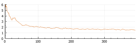
During training, the current loss value is shown both numerically and in the Loss curve, which plots loss (y-axis) against iterations (x-axis). As training progresses, the loss is expected to decrease and eventually stabilize. Training can be stopped when the loss curve has converged, i.e., when it remains stable over several iterations. It is recommended to pause training periodically and preview the APP to assess performance and ensure that learning progresses as expected.

note

When continuing training with new images that were not previously included, a temporary increase in the loss curve is expected. This occurs because the model encounters new variability it has not yet learned. As training continues, the loss should decrease again as the model adapts.

To delete the training, open the dropdown menu on the Train/Stop/Continue button and select Delete training .

The Probability Setting

The Probability value, controlled by the slider, defines the minimum probability required for a pixel to be assigned to an image class. A pixel is classified as the class with the highest probability, provided that this probability exceeds the selected threshold. For example, consider a pixel with probabilities of 40% for class A, 35% for class B, and 25% for class C. If the minimum probability is set to 50%, the pixel will remain unclassified. If the threshold is set below 40%, the pixel will be assigned to class A. The default probability is 0%, meaning that all pixels are classified according to the class with the highest probability.

The loss curve

The training plot visualizes how the model performance evolves during training. It is commonly referred to as the loss curve, as loss is the default measure shown. However, the plot can also display another metric (the error rate), and can therefore be more generally described as a convergence curve.

The x-axis shows the number of iterations, while the y-axis shows the selected performance measure (e.g., loss or error rate). The displayed measure can be changed using the dropdown menu next to the training plot icon .

Loss is the primary measure used during training to optimize the neural network. It quantifies the difference between the model’s predictions and the true labels as a single scalar value. As training progresses, the loss is expected to decrease, indicating that the model is improving. When training is paused or stopped, the latest loss value is displayed both in the plot and next to the network architecture.

Example of a loss curve showing a loss of 0.071 after 394 iterations.

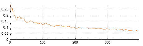
Metric (Error Rate). A metric is used to evaluate model performance in a more interpretable way. In this case, the metric is the error rate, expressed as a percentage of incorrectly classified pixels. The error rate typically fluctuates during training but generally decreases as the model improves. Like loss, the current value is shown when training is paused or stopped.

Example of a convergence curve showing an error rate of 1.5% after 394 iterations.

Iterations represent the number of times batches of training data have been processed by the model. The number of iterations is shown along the x-axis of the training plot and next to the current loss or metric value.

Features from Deep Learning

After training a Deep Learning classifier, a feature for each defined image class appears under the Features subsection in the Classification section. Each feature represents the probability that a pixel belongs to the corresponding image class, and the sum of all feature values (probabilities) is therefore equal to one for each pixel. These features are the output of the deep neural network. The classifier uses them to assign each pixel to the class with the highest probability. To preview a feature, click the eye icon to the right of the feature. The result is displayed in the current field of view (FOV). This causes the deep neural network to compute the selected feature. While previewing, hovering over a pixel reveals its exact probability value.

Previewing the glomerulus feature in a glomerulus detection app: at the pixel marked in red, the probability of that pixel belonging to the glomerulus class is approximately 81.3%

tip

It is possible to apply filters to these features, as with any other feature. However, doing so means the probabilities will no longer sum to one. For advanced users, a different classifier can be applied after training. The features are still computed by the deep neural network (which is saved with the APP), and another classifier (e.g., a Threshold classifier) can be used to perform the final classification. For general information on features, see the Define Image Features section.

Tensorboard integration

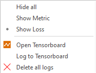
TensorBoard is an open-source tool from Google that can be used to visualize training progress. It is possible to send training information from a Visiopharm installation directly to TensorBoard. TensorBoard options are available from the dropdown menu next to the training plot icon .

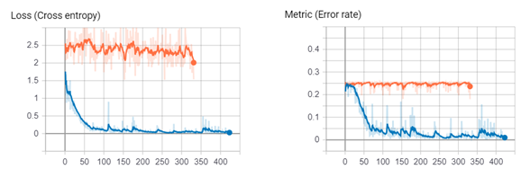
TensorBoard serves as an alternative to the simple training plot (showing the loss curve) for inspecting the progress of a deep neural network. It provides access to both metric (error rate) and loss function curves, where the loss function represents how well the model matches the training data and is the value that is minimized during training. In addition, TensorBoard enables saving of training sessions, which allows comparison of multiple runs where for instance the learning rate is adjusted.

An example of the loss and metric (error rate) curves from two seperate training sessions in Tensorboard is shown below, illustrating the training progress of two separate deep neural networks.

The loss- and metric (error rate) function curves of two separate training sessions with different learning rates (orange: low learning rate. blue: higher learning rate).

Opening Tensorboard

1. Click Open Tensorboard from the dropdown menu. This will start Tensorboard and opens the client in the default browser.

2. Select Scalars in the TensorBoard ribbon to view training curves (e.g., loss function and metric (error rate)). If the Scalars tab is not visible, ensure that training is currently running.

3. Select Graphs in the ribbon of Tensorboard to view how the selected neural network is designed. This view also allows comparison between available network architectures (see the Network Architectures section).

Error Handling and Common Pitfalls

Even when following the recommended workflow, issues may occur during training or application of a Deep Learning APP. This section highlights common pitfalls and how to resolve them.

General considerations

Running an APP overwrites training labels. When an APP is executed, the resulting classification replaces any existing training labels. To avoid losing annotations, it is recommended to create a copy of the image with the drawn labels and run the APP on the copy instead.

Some changes require retraining. While it is common to add new images and continue training, certain changes require the network to be retrained from scratch. These include:

• Adding or removing image classes
• Changing input channels
• Adjusting magnification (while it is possible it is not recommended after training)

To avoid unnecessary retraining, ensure that image classes, labels, input channels, and magnification are correctly defined before starting training.

Input configuration issues

Correct input configuration is essential for successful training. For standard brightfield images, the input channels are typically Red, Green, and Blue (RGB). For other image types, the required input channels may differ depending on the imaging setup. In either case a maximum of three input channels can be used for training.

important

If training fails to start:

• Verify that no more than three input channels are selected.

Input settings can be configured under AI Architect - Advanced deep learning settings, accessible by clicking on the icon.

Select Inputs dialog

The Select Inputs dialog appears when the APP expects input channels that are not defined in the image. This is indicated by the message:

“APP cannot run because the image's color setup is different from what the APP expects.”

Select Inputs dialog.

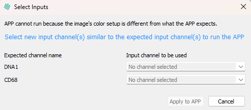
To resolve this, assign the appropriate image bands to the expected channels using the dropdown menus. For example, select the image band corresponding to DNA1 if required.

Converged training but poor results

If the training loss has stabilized but the classification results are unsatisfactory, further training with the same setup is unlikely to improve performance. In such cases, consider the following:

• Add more training data. Increasing the number and variability of training examples often improves performance.

• Refine results with post-processing. If objects are generally detected correctly but boundaries are inaccurate or noisy, implementing Post Processing steps can improve the final result.

• If the above steps are insufficient, consider adjusting model settings. Modifying network or training parameters, as described in the AI Architect - Advanced deep learning settings section, may further improve performance.

info

If issues persist, contact Visiopharm support at support@visiopharm.com.