Deep Learning Models and Network Architectures

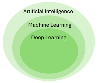
This section provides a conceptual, high-level introduction to how deep learning models for image segmentation work. Deep learning models are a subgroup of machine learning models. In broad terms, they are mathematical models that learn patterns directly from data. What distinguishes deep learning from other machine learning approaches is the use of neural networks-model architectures originally inspired by the way biological neurons are organized (hence the name).

A neural network consists of a set of interconnected neurons arranged in layers: an input layer, one or more hidden layers, and an output layer. The term deep refers to the use of multiple hidden layers, which allows the model to learn increasingly complex patterns in the input data. Patterns are learned progressively: each layer processes the information it receives, extracts relevant features, and passes the result to the next layer, building increasingly abstract representations up to the output layer.

There are many different types of deep learning models, designed for different problem domains. Examples include large language models (such as ChatGPT) and image-based models for tasks such as classification. In the context of Visiopharm, deep learning is used for image segmentation and classification in medical image analysis. The models employed by Visiopharm are semantic segmentation models designed specifically for medical image analysis, and it is therefore these types of models that are conceptually explained in this section.

Basic Deep Learning Pipeline

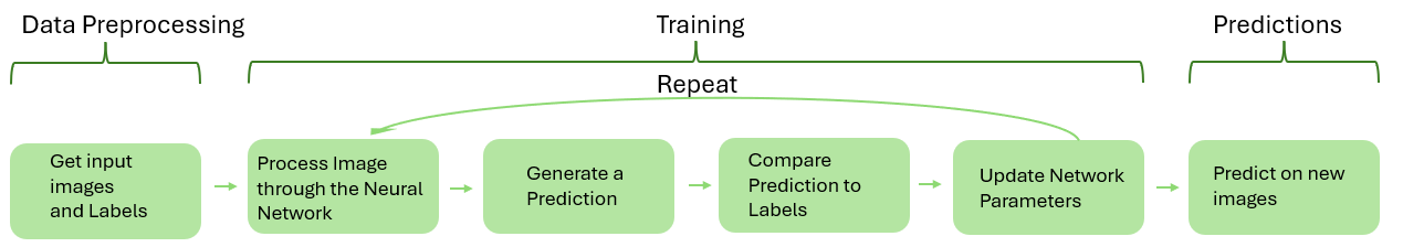
The deep learning models utilized in Visiopharm are supervised models, meaning they are trained using labeled data that explicitly indicates what different structures or objects in an image represent. During training, the model learns to associate image features with the provided labels. This training is an iterative process, which continues until the model has learned sufficiently from the labeled data to produce satisfactory predictions. Below is a schematic overview of the supervised deep learning workflow, showing the process from data input and preprocessing through iterative training to final predictions.

1. Get input images and labels The first step in the pipeline is to obtain suitable training data for the deep learning model. For example, if the objective is to create a deep learning APP that can distinguish tumor from stroma in lung tissue, the input data should consist of multiple lung tissue images that accurately represent the tissue types to be analyzed. These training images are then labeled, such that each pixel in an image is labeled according to its class (e.g., tumor or stroma). For a detailed description of the labeling process, see Using Deep Learning in Visiopharm. Before training, the images typically undergo data augmentation, which can be configured in the AI Architect. Data augmentation artificially increases variation in the training data (for example through rotation, scaling, or color variation) to improve model robustness and generalization.

2. Process the images through the neural network Training begins by feeding the input images (not the labels) through the neural network. Using its internal parameters, referred to as weights the network extracts features from the images. These features may include low-level characteristics such as edges or color intensities, as well as higher-level patterns that help distinguish tissue types. The initial weights are determined through pretraining performed by Visiopharm. As training progresses, the weights are continuously updated based on how well the model's predictions match the labeled data, enabling the network to extract increasingly relevant features from the images (step 5.). The exact way images are processed depends on the network architecture, which is described further in the Network Architectures section below.

3. Generate a prediction Once an input image has passed through all layers of the network, the final output is converted into a set of class probabilities for each pixel. For a Tumor/Stroma Classifier, the model would assign a probability that a given pixel belongs to tumor tissue versus stroma. For each pixel, the class with the highest probability is selected as the model's prediction. This pixel-wise classification of the entire image is what defines the approach as semantic image segmentation.

4. Compare predictions to the labels The predicted output is then compared to the corresponding drawn labels. The discrepancy between the predictions and the correct labels is quantified using a loss function, which measures how well the model is performing. A high loss indicates that many pixels are incorrectly classified, while a low loss indicates better performance. The loss is typically tracked over training iterations and visualized as a loss curve.

5. Update the model weights Based on the computed loss, the model's weights are adjusted to reduce the error. This adjustment is performed using backpropagation, in combination with a chosen optimizer. The learning rate controls how much the weights are updated at each iteration: a higher learning rate results in larger updates, while a lower learning rate leads to more gradual changes.

6. Repeat the process Steps 2-5 are repeated for many images and across multiple training iterations. Over time, the model gradually improves its predictions as it learns more robust and relevant representations from the data.

7. Predict on new images Once training is complete, the trained model can be applied to previously unseen images. The model generates predictions based on the features and patterns it has learned during training, for example identifying which regions correspond to tumor and which to stroma.

Network Architectures Supported in Visiopharm

Visiopharm supports three deep neural network architectures for semantic image segmentation: U-Net (default), DeepLabv3+ (Requires GPU), and FCN-8s. The choice of architecture determines how input images are processed through the neural network and how spatial and contextual information is extracted and combined.

While many different deep learning architectures exist for semantic segmentation, they often share common structural components. These typically include the use of convolutional neural networks (CNNs) as feature extractors, an encoder-decoder design, spatial downsampling and upsampling operations, and skip connections to preserve spatial detail.

The following section describe architectural concepts and operations that are common to all three architectures supported in Visiopharm. Although the underlying principles are shared, the specific implementation and degree to which each concept is used varies between models.

Common Architectural Concepts

Most segmentation architectures follow an encoder-decoder design. The encoder progressively reduces the spatial resolution of the input image while extracting increasingly abstract and semantic features through convolution and downsampling operations. The decoder then restores the spatial resolution using upsampling operations, producing a pixel-wise segmentation map. To retain fine-grained spatial information that may be lost during downsampling, skip connections are often used to transfer feature maps from the encoder directly to corresponding stages in the decoder.

In all supported architectures, the network can be conceptually divided into an encoding stage that extracts semantic features and a decoding stage that produces dense, pixel‑wise predictions, even if the architectural implementation differs between models.

Image representation (pixels, channels)

A digital image is represented as a grid of pixels, where each pixel encodes color intensity values. For grayscale (Black and white) images, each pixel contains a single intensity value (e.g. 0 = black, 255 = white). For RGB (Color) images, each pixel consists of three values corresponding to the red, green, and blue color channels. These pixel intensity values form the numerical input that is processed by the neural network.

Encoder-decoder structure

Most semantic segmentation networks follow an encode-decoder structure. The encoder progressively reduces the spatial resolution of the input image while extracting increasingly abstract features. All supported architectures use several encoder layers, each of which makes use of convolutions to downsample the image and extract a feature map. Early encoder layers capture simple structures, while deeper layers learn more complex patterns in the input data.

The purpose of the encoder layers is therefore to extract the elements of the image that are meaningful for the task at hand. For a simple tissue detection, the difference in pixel intensity between the tissue and background, or the edges of the tissue objects, could for instance be meaningful for the model to learn in order to distinguish future tissue from background. In practice, however, the features extracted by the encoder layers do not translate directly to an easily interpretable feature list. Instead, each layer outputs a feature map. This feature map is the model's way of compressing the input image into just the meaningful features that help it distinguish the different classes it needs to classify. The feature map is a matrix with dimensions that are typically smaller than the image dimensions inserted into the encoder layer. This feature map is then passed into the next encoder layer, which extracts even more complex features, and so on.

After the final encoder layer, the decoder then reverses this process by gradually restoring spatial resolution through upsampling operations. Using the learned high-level features from the encoder, the decoder produces a dense, pixel-wise segmentation map that aligns with the original image size.

Convolutions

Convolutional operations are the fundamental building blocks of all three architectures supported in Visiopharm. These operations apply small, learnable filters called kernels across the input to extract local features such as edges, textures, and shapes.

Convolution example: a kernel is applied to each pixel in the image, and for each pixel (for instance f), it computes an output depending on the surrounding pixels and f, for example aw11 + bw12 + cw33 + ··· + kw33. This output is then inserted into the corresponding position of the resulting feature map.

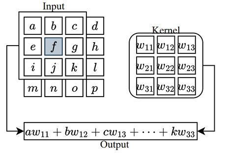
As illustrated in the above figure, the convolution operation involves applying a kernel to a localized region of the input image. At each position, the kernel values are in this case multiplied element-wise with the corresponding input values, and the results are summed to produce a single scalar value that is inserted into the resulting feature map. This process is repeated as the kernel moves across the input, systematically producing the complete feature map.

Several key parameters influence this operation. The kernel size determines the spatial dimension of the region processed at each step. The stride defines the step size with which the kernel shifts over the input and therefore also the downsampling of the feature map compared to the input image. Finally, the entries of the kernel itself (the weights) determine the scalar output. It is these weights that are iteratively updated during training, as detailed in steps 2-6 of the basic pipeline.

Upsampling and downsampling

Up- and downsampling are the operations that allow the image resolution (the input at each encoder/decoder layer) to be compressed and restored to selected sizes. Downsampling can be implemented using pooling operations or strided convolutions, depending on the architecture. Max pooling is one commonly used technique, illustrated below. Pooling operations serve to reduce the spatial dimensions of the feature maps while retaining important information. In max pooling specifically, each local region is replaced by its maximum value, effectively preserving the strongest feature signals while discarding less relevant ones. Similarely average pooling would preserve the averge feature signal, etc.

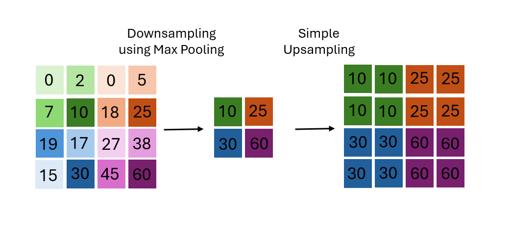
A simple upsampling technique is then equivalently to enlarge the resolution by multiplying each input pixel into a 2 by 2 grid to restore the resolution.

Skip connection

The encoder-decoder structure described so far repeatedly downsamples the image and then upsamples it again. While this allows the model to learn increasingly abstract features, it also results in a loss of fine spatial detail. This loss occurs because the features extracted in deeper layers are based on increasingly large regions of the image, causing them to become detached from the original spatial context. To address this, skip connections are introduced. Skip connections transfer high-resolution feature maps from the encoder directly to the decoder. Specifically, they pass the feature maps from an encoder layer to the corresponding decoder layer of the same spatial size. While the encoder continues to extract more abstract, high-level patterns, the skip connections preserve the detailed spatial information from earlier layers. This allows the decoder to combine coarse semantic understanding with fine-grained spatial structure. As a result, the model is better able to both identify what is present in the image and accurately localize where it is, leading to improved segmentation performance.

---

Together, these architectural concepts define a common framework for semantic image segmentation in Visiopharm. All supported models transform pixel-level image data into semantic feature representations through convolution and downsampling, and then reconstruct pixel-wise predictions through upsampling by combining information learned at different stages of the network.

The difference between FCN-8s, U-Net, and DeepLabv3+ lies not in whether these concepts are used, but in how they are realized and emphasized. FCN-8s represents a foundational segmentation architecture with a simple design. U-Net extends this approach with a fully symmetrical encoder-decoder structure and dense skip connections, making it well suited for applications requiring high spatial precision. DeepLabv3+ focuses on looking at the image simultaneously at different spatial scales to understand both fine details and larger structures, trading architectural symmetry for efficiency and improved handling of large or complex structures.

The following sections describe each architecture in turn, highlighting how the shared concepts introduced above are implemented in practice.

FCN-8s

The Fully Convolutional Network (FCN) was one of the first deep learning architectures designed specifically for pixel-wise image segmentation, rather than image-level classification. Unlike classification networks, which output a single label for an entire image, FCN architectures produce a prediction in which each pixel is assigned a class label.

Network structure of FCN-8s. The leftmost white square represents the input image. The sequence of green and purple squares illustrates the encoding path, where the image is processed through convolution and pooling operations, gradually reducing its resolution. The white squares on the right show the decoder path, where the resolution is increased again. Skip connections link feature maps from earlier layers at 1/32, 1/16, and 1/8 of the original image resolution, allowing the network to combine coarse and fine information when producing the final segmentation.

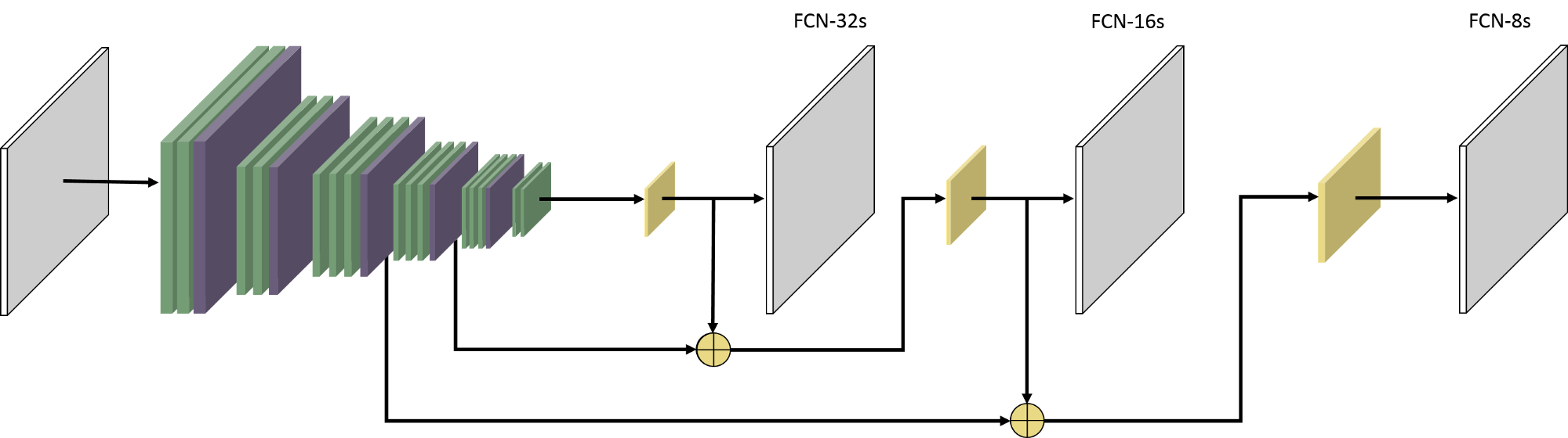
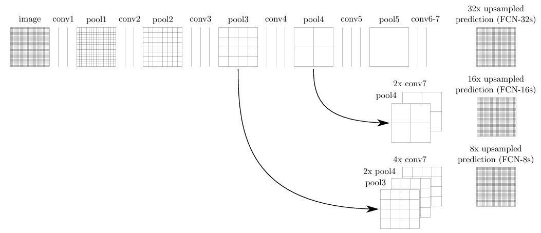
In FCN-8s, the input image is gradually reduced in size as it passes through several convolutional and pooling layers. At its deepest point, the image representation is only 1/32 of the original resolution. This low-resolution representation captures the overall content of the image, but lacks fine detail. To produce a full-resolution segmentation, the network increases the resolution again. A simple approach (FCN-32s) would be to upscale directly from this coarse representation, without including any skip connections to add spacial context. FCN-16s improves this by incorporating information from an earlier layer where the image is still at 1/16 of its original size. FCN-8s goes one step further by also including information from a layer at 1/8 of the original resolution. These skip connections, allow the model to combine coarse, high-level information with finer spatial details from earlier layers. As a result, FCN-8s produces more precise segmentations than simpler variants that rely only on the deepest layer. However, it remains a relatively simple architecture and is primarily used as a foundational model. More advanced methods, such as U-Net and DeepLabv3+, build on these ideas to achieve higher accuracy and better handling of fine spatial details. For further technical details, see the original FCN paper by (Long, Shelhamer, & Darrell 2015). The network architecture as proposed in the original paper is shown below.

The proposed model FCN-8s learn to combine coarse, high layer information with fine, low layer information. Pooling and prediction layers are shown as grids that reveal relative spatial coarseness, while intermediate layers are shown as vertical lines. First row (FCN-32s): The single-stream net, upsamples stride 32 predictions back to pixels in a single step. Second row (FCN-16s): Combining predictions from both the final layer and the pool4 layer, at stride 16, lets the net predict finer details, while retaining high-level semantic information. Third row (FCN-8s): Additional predictions from pool3, at stride 8, provide further precision.

U-Net (Default)

U-Net is a convolutional neural network architecture originally developed for biomedical image segmentation.

Network structure of U-Net.

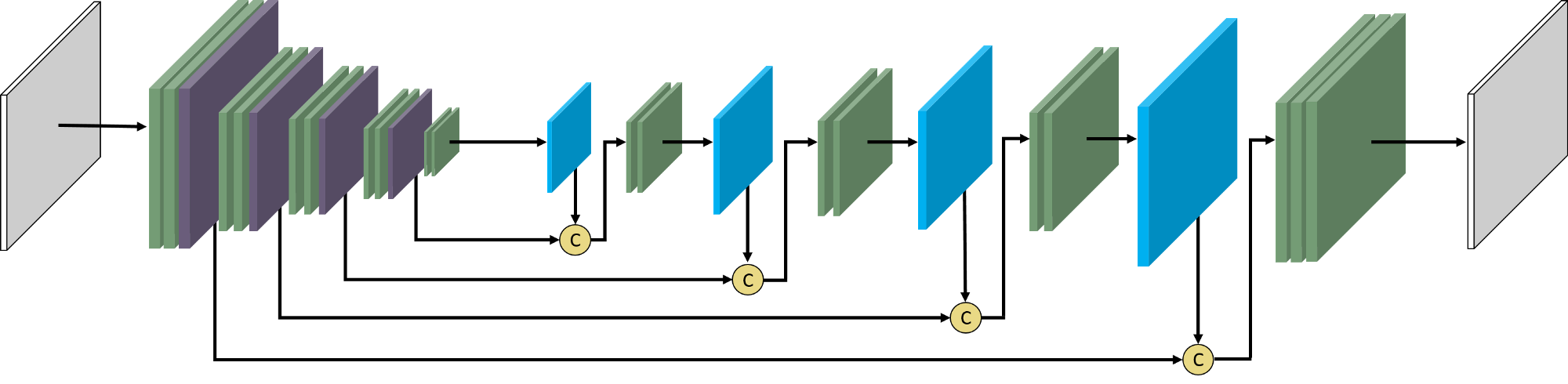
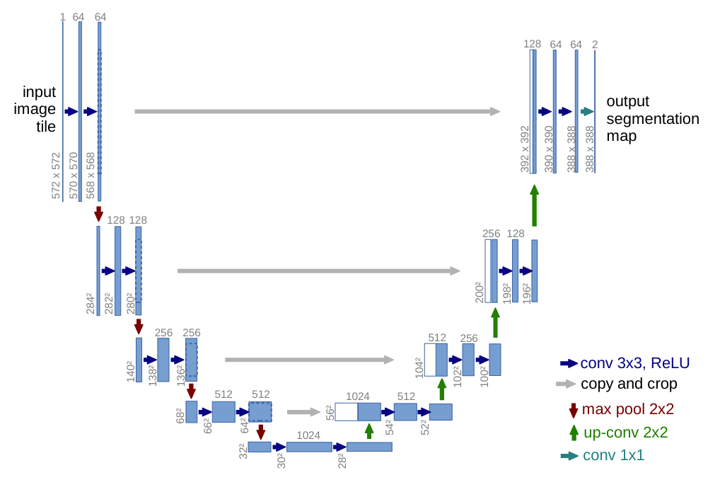
It is characterized by a symmetric encoder-decoder structure with skip connections, forming a U-shaped layout (best seen in the figure proposed in the original paper below).

The encoder gradually reduces the resolution of the input image through convolution and pooling operations, allowing the model to learn increasingly abstract features. However, this process also removes spatial detail. To address this, the decoder path progressively restores the image resolution. At each stage, skip connections transfer high-resolution features directly from the encoder to the decoder. This allows the model to retain detailed spatial information while still benefiting from the high-level understanding learned in deeper layers.

Compared to FCN-8s, U-Net makes more systematic use of skip connections throughout the network, allowing it to better preserve fine spatial details during reconstruction. As a result, U-Net generally produces more accurate and detailed segmentation outputs.

For this reason, U-Net is commonly preferred over FCN-based models and is used as the default architecture in Visiopharm. For further details, see the original paper by (Ronneberger, Fischer, & Brox 2015). The network architecture as proposed in the original paper is shown below.

U-Net architecture as shown in the original paper. Blue boxes represent feature maps at different resolutions. Skip connections (grey arrows) copy information from the encoder to the decoder at matching resolutions.

DeepLabv3 (Requires GPU)

Network structure of DeepLabv3+. The input image is first processed by an encoder (top), where atrous convolutions are used to extract features. Multiple parallel convolutional layers with different dilation rates (Atrous Spatial Pyramid Pooling, ASPP) capture information at different scales. The outputs are combined and passed to the decoder (bottom). Low-level features from earlier layers are reintroduced to refine object boundaries. The resolution is then gradually restored before the final prediction.

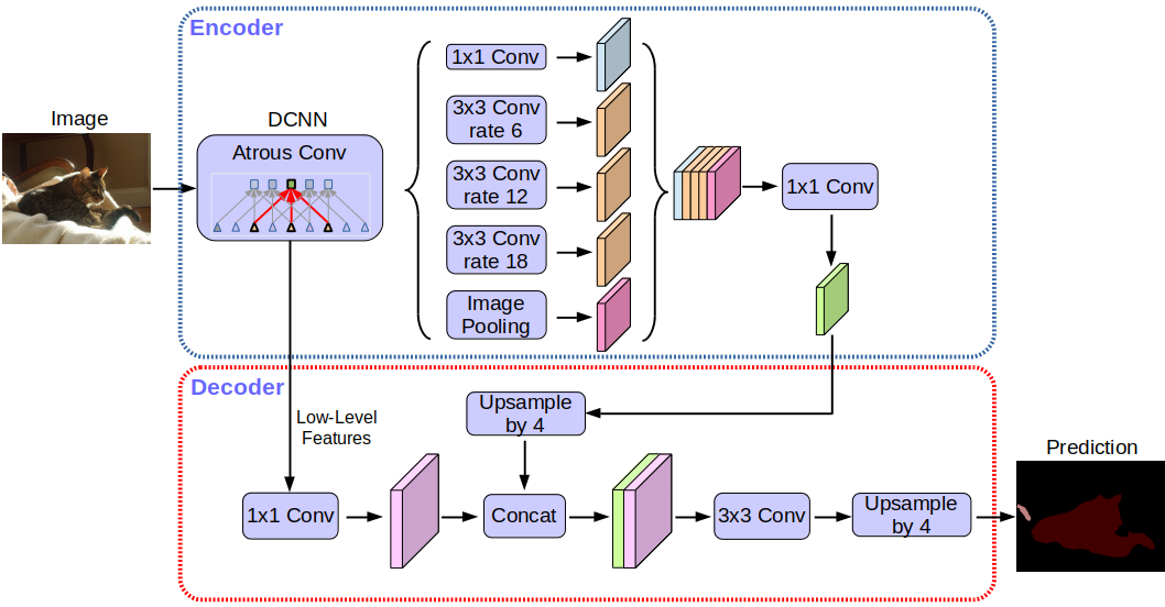
DeepLabv3+ is an advanced segmentation architecture that builds on ideas introduced in FCN, U-Net, and other approaches. Like these models, it combines high-level semantic information with spatial detail, but does so in a more efficient and flexible way.

In the encoder, DeepLabv3+ uses atrous (dilated) convolutions, which allow the network to capture a larger area of the image without reducing the resolution as much as traditional pooling. This helps preserve spatial detail while still capturing global context.

A key component of DeepLabv3+ is the Atrous Spatial Pyramid Pooling (ASPP) module. Instead of relying on many skip connections or repeated downsampling and upsampling, ASPP processes the image using several parallel filters at different scales. This allows the network to capture both fine details and broader contextual information at the same time.

The decoder then refines the segmentation by combining these features with information from earlier layers. Compared to U-Net, this decoder is simple but efficient, requiring fewer upsampling steps while still improving the accuracy of object boundaries.

As a result, DeepLabv3+ often produces more accurate and robust segmentation results than both FCN-8s and U-Net, particularly in complex images where objects appear at different scales. However, because the architecture is more complex, it requires more computational resources, specifically a GPU, when used in Visiopharm.

For further details, see the original paper by (Chen et al. 2018).

Comparison of Architectures

U-net	DeepLabV3+
Good at segmenting small structures (nuclei etc.) with high detail level.	Good at segmenting large, size-varying structures. More Context based.
Slower convergence and slower runtime (compared to DeepLabv3+).	Faster convergence and faster runtime (compared to U-net).
Default framework in VIS. Originally developed for medical image segmentation.	Segmentation results are smoother and more precise around the object boundaries (compared to U-Net).
Example application: Nuclei Detection.	Example application: Detection of Metastatic areas Tumor/stroma separation.

Sources

This section is primarily based on the original papers introducing the three architectures: FCN-8s, U-Net, and DeepLabv3+.

The original FCN-8s paper by Long, Shelhamer, & Darrell 2015.

The original U-Net paper by Ronneberger, Fischer, & Brox 2015.

The original DeepLabv3+ paper by Chen et al. 2018.

The basic deep learning pipeline and architectural concepts presented here are loosely inspired by the book Deep Learning by Ian Goodfellow, Yoshua Bengio and Aaron Courville. However, the explanations in this documentation are simplified and adapted to make them accessible to non-technical users and readers without prior experience in machine learning.