Deep learning

Deep learning Method in the Classification section of the APP author.

Deep learning and convolutional neural networks are a broader family of AI machine learning methods. It involves neural network algorithms that use a cascade of many layers of nonlinear processing units for feature extraction and transformation with each successive layer using the output from the previous layer as input. Using deep learning for classification allows you to segment abstract image structures that would be impossible to segment with a simple pixel classifier.

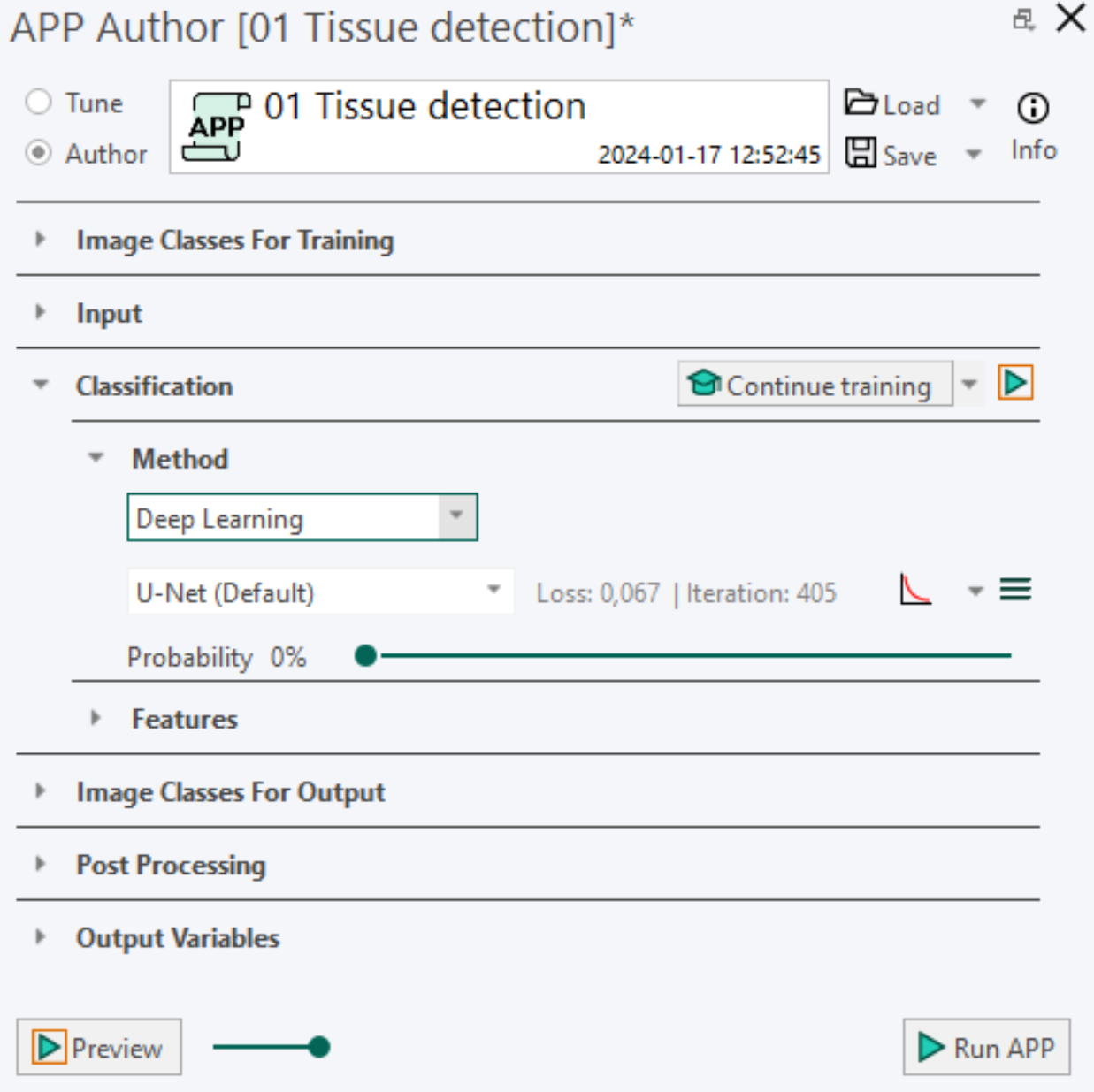
Network Architecture U-Net (Default), DeepLabv3+ (Requires GPU) and FCN-8s are three different network architectures. We generally recommend choosing U-Net over FCN-8s and DeepLabv3+, which is emphasized by the (Default) tag.

Convergence Curve is a simple training plot showing the learning performance of the neural network. The x-axis shows the number of iterations, while the y-axis shows the training loss or error rate depending on the settings. The settings are found in the dropdown menu of the training plot icon .

Loss is a measure used determine the performance of the network optimization algorithm to a scalar value by measuring the inconsistency between predicted and actual values. The robustness of the model increases with the decrease of training loss. When the training is paused or stopped, the final loss value is shown. The training loss is available from the dropdown menu next to the training plot icon . When selected, the loss of the network is visualized in the training plot and next to the network architecture.

An example of a convergence curve with a loss of 0.071 after 394 iterations.

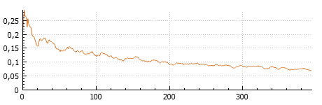
Metric is a measure used to evaluate the network algorithm. The performance metric used is the error rate. The error rate percentage fluctuates and decreases during training until the model has converged. When the training is paused or stopped, the final error rate percentage is shown. The training metric is available from the dropdown menu next to the training plot icon . When selected, the error rate of the network is visualized in the training plot and next to the network architecture.

An example of a convergence curve with an error rate of 1.5 % after 394 iterations.

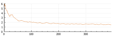
Iterations are the number of times a batch of data has passed through the network algorithm. The number of iterations are visualized in the training plot and next to the training loss or error rate.

Probability value is determined by the slider position indicates the minimum probability needed in order to classify a pixel as one of the image classes. The deep learning classifier will classify a pixel to the class having the highest probability, given that it is above this minimum value. As an example, consider a pixel having a probability of 40% for belonging to class A, 35% for class B and 25% for class C. If the minimum probability value is set to 50%, the pixel will not be classified as any of the classes. On the contrary, if a value below 40% is chosen, the pixel will be classified as class A.

Advanced Deep learning settings By pressing the menu button of the APP author, the AI Architect dialog appears for advanced deep learning settings.

Tensorboard is an open-source tool from Google, and we send information about training progress from your Visiopharm installation to Tensorboard. Tensorboard options are available from the dropdown menu next to the training plot icon .

Select Inputs dialog

Select Inputs dialog

This dialog is opened when certain APPs are launched, where some color bands have yet to be defined, as indicited in the message: "APP cannot run because the image's color setup is different from what the APP expects."

Select Inputs dialog.

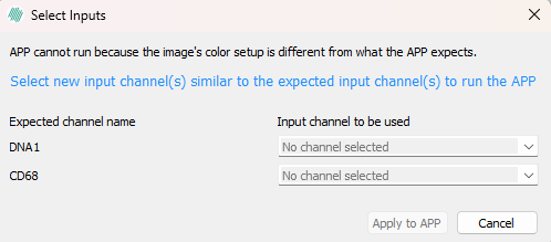
To resolve this, simply select bands in the image from the dropdown menu that correspond to the Expected channel names, eg for DNA1 select the band in the image that contains this biomarker.

Network Architecture

All deep learning models in Visiopharm are so-called semantic segmentation networks, that utilize deep convolutional neural networks (CNNs). Most of the models use a VGG-style (Simonyan & Zisserman, 2014) encoder as backbone CNN. Here we cover U-Net (default), DeepLabv3+, FCN-8s, and a Comparison of U-net and DeepLabV3.

U-Net (Default)

Network structure of U-net

U-Net drops the last two layers of VGG in order to speed up the computation. The U-Net concatenates the information of the previous tensor and the up-sampling tensor rather that using element-wise addition to fusion the information. This is two advantages of the U-Net compared to the FCN network. The tensor will also get through two convolution layers to reinforce the intensity after each up-sampling operation. We generally recommend using the U-Net network architecture over the FCN-8s architecture. For more information about U-Net, see the original paper (Ronneberger, Fischer, & Brox 2015).

DeepLabv3+ (Requires GPU)

Network structure of DeepLabv3+

DeepLabv3+ use atrous spatial pyramid pooling (ASPP) module augmented with image-level feature to capture feature information on different scales. This means that instead of use step-wise upsampling blocks to incorporate features from different levels, this network only needs two upsampling steps, i.e. it is faster to train and analyze than e.g. the U-Net. All of this also means that the decoder module can refine the segmentation results along the object boundaries more precise. For more information on the DeepLabv3+ network architecture please refer to the original paper (Chen et al. 2018).

FCN-8s

Network structure of FCN-8s

The FCN (fully convolutional network) originates from a desire to segment objects in pixels instead of just object recognition. It processes the image through the network and produces the course feature response map at the end, which will be up-sampled. The FCN-8s means that the result is shrank 8 times of the original image and it gets through two up-sampling layers and element-wise additions. For more information on FCN-8s network architecture, please refer to this paper (Long, Shelhamer, & Darrell 2015).

Comparison of U-net and DeepLabV3+

U-net	DeepLabV3+
Good at segmenting small structures (nuclei etc.) with high detail level.	Good at segmenting large, size-varying structures. More Context based.
Slower convergence and slower runtime (compared to DeepLabv3+).	Faster convergence and faster runtime (compared to U-net).
Default framework in VIS. Originally developed for medical image segmentation.	Segmentation results are smoother and more precise around the object boundaries (compared to U-Net).
Example application: Nuclei Detection.	Example application: Detection of Metastatic areas Tumor/stroma separation.

Getting started

Here we cover how to create a Deep Learning APP, how to train a Deep Learning Classifier, understanding features in repspect to Deep Learning, as well as how to use Tensorboard.

Create a Deep Learning APP

For this guide, we aim for an APP that is able to automatically detect glomeruli, which are small structures in the kidneys shown in the image below.

Detecting glomeruli shown in this image is the example task (Kidney CD68).

1. Create a new APP by pressing the New APP button in the Image Analysis section in the ribbon.

2. Create an image class in the Image Classes for Training section for each desired image structure and/or a background class. The background class needs to be positioned in the top of the image class list if training labels are to be drawn inside a ROI. In this example, we have a single type of image structure to detect, glomeruli, and thus we will have a total of two classes including the background class.

3. Draw training labels on all cases of the image structure of interest (glomeruli) in the entire training slide(s). In this case, it means that every glomerulus should be labeled, and some descriptive examples of the background class should be drawn. If ROI's are not drawn on the slide then only pixels with training labels are used for training.

   If ROI's are drawn on the slide, all pixels within the ROI will be used for training. Pixels not marked with labels are assumed to be the first training label, which in this case is Background. However, to guide the sampling, it is required that you provide at least one example of the background class, i.e. draw at least one background training label. Drawing a too small ROI can reduce the size of the data set to the point where the model will overfit, resulting in wrong predictions. Avoid drawing ROIs that go through an object, as this will teach the algorithm that the object should be bisected. Additionally, avoid drawing labels outside of ROIs, as this will interfere with training.

4. Setup the Input section with a desired magnification.

5. Under the Classification -> Method, select Deep Learning as the classifier. Leave the settings at the default settings (U-Net (Default), Probability= 50%)

6. Press the train button to start training the APP. After a short delay, the error rate shown to the right of the network architecture name will fluctuate and decrease.

7. While the APP is training, you can click on the training plot icon if the convergence graph is not visualized. When the training seems to have converged, you can stop the training by clicking the stop button.

8. Save the APP in order to save the APP together with the trained neural network by pressing the save button .

9. Preview/Run the APP. Previewing the APP will classify the FOV and is done by pressing the preview button in the bottom of the APP Author dialog. Running the APP will classify the entire slide.

Training a Deep Learning Classifier

Before commencing the training process of the classifier, make sure that all statements on the checklist beneath are true:

• Each type of object you want to detect in your image has its own image class in the Image Classes for Training section in the APP author.
• The background image class is always the uppermost class in the Image Classes for Training list in the APP Author.
• Each training slide/image contains one or multiple training ROIs.
• Every object of interest present in the training ROI(s) in the image is labeled as its corresponding image class.
• At least one label of every class is drawn inside a training ROI.

Setup Image classes for training. All image classes (labels) that you want the Deep Learning classifier to detect need to be specified in the Image Classes for Training section in the APP Author dialog. A background class needs to be added as well and should always be on the top of the list of the classes in the Image Classes for Training section. The reasoning behind is that the Deep Leaning classifier assumes the first element in the Image Classes for Training is the "background" class. For example, if you want to create a Deep Learning classifier which can detect Ki-67-positive and Ki-67-negative nuclei in a Ki-67 IHC slide, you will need a total of three image classes, e.g., Background, Positive nucleus, Negative nucleus. Adding an additional image class to an APP after the network has been trained will result in the deletion of the training results and requires a retraining of the APP. Make sure to always save your APP during training and before making any changes.

Draw training labels. The optimal way to setup training labels to train a Deep Learning network is by using training ROIs in images. Start selecting an area(s) in the image(s) you want to use for training and draw ROI(s). Now, draw training labels corresponding to your Image Classes for Training inside the ROI(s). Make sure to label every class carefully within the training ROI(s) which doesn't belong to the background class, because the algorithm assumes that every unlabeled pixel belongs to the background image class. Otherwise, the training algorithm may receive cases of an image class (e.g., glomeruli, nucleus, or necrosis) wrongly labeled as the background class, which causes the network to segment image structures of interest as the background class. It is still required to have one background label in the image(s) to start the training. We recommend including one small example of background label in each training ROI. To train a well performing Deep Learning classifier, it is important to include the variability of the image classes by adding multiple training ROIs and labels. As rule-of-thumb, start with at least 2-4 squared training ROIs at the size of the FOV per image. Note that the number of training ROIs needed for a sufficient training result is strongly dependent on the inherited tissue variation the Deep Learning network needs to learn. Ensure that no training labels are drawn outside the ROIs, as this will result in these labels being masked as in the Masking preproccesing step, and then being used for training, which might result in incorrect training.

Training labels without ROIs. The Deep Learning classifier can also be trained using training labels without drawing training ROIs. Be aware that this way of labeling is generally not recommended as this will lead to a lack of contextual information during the Deep Learning training. Labeling without training ROIs cause the Deep Learning classifier to ignore the unlabeled pixels during the training

Start / Stop Training Process. The training process of a deep neural network is an iterative process optimizing an extreme number of parameters. The training process is started by pressing the Train button in the APP Author dialog . The training process may run for a very long time while the Deep Learning classifier becomes better and better. The process can be stopped at any time by pressing the Stop button and can be continued by pressing the Train button again, which thereby allows continuing the training with additional training data. During the training, the current loss value can be seen directly in the loss field and on the convergence graph, which shows the loss value (y-axis) by the number of iterations (x-axis). Do not zoom in/out on the image while training, it will stop the process. The training can be stopped when the loss graph has converged i.e., when the loss value becomes stable for several iterations. We recommend that you pause the training regularly and preview the APP to get a feel for its progression.

tip

To train on several images use Ctrl+Click to select all the images you wish to train on and select "Train" or "Continue train" under classification.

Features from Deep Learning

After training a Deep Learning classifier, a feature for each defined image class will appear under the Features subsection in the Classification section. Each feature represents the probability that a pixel belongs to the corresponding image class, and the sum of all feature values (probabilities) thus sum to one for each pixel. These features are the result of the Deep Neural Network. The Deep Learning classifier uses these features, resulting from the deep neural network, to classify each pixel to the class having the highest probability.

If you want to preview any of the features, click the eye icon to the right of the feature, and the feature will be previewed in the current field-of-view. This will make the deep neural network compute that feature.

It is possible to add filters to the features, as with any other features, however, keep in mind that the probabilities thereby will no longer sum to one. For the advanced users, it is also possible to choose another classifier after training your network. The features are still computed from deep neural network (which is saved with the APP), and then e.g. an Threshold classifier could be used to perform the actual classification.

While previewing a feature, you can hover the mouse pointer over a pixel in the field-of-view to see the exact probability value.

Tensorboard Integration

Tensorboard is an alternative to the simple training plot used to inspect the training progress of your deep neural network. Here, you can see both metric (error rate) and loss function curves, which is the underlying function that is used in the training. It will save the session, so you can compare training curves, and e.g. use it to guide adjustment of the learning rate.

An example of the loss- and metric (error rate) function curves of two sessions in Tensorboard have been visualized below, showing the training progress of two separate deep neural networks.

The loss- and metric (error rate) function curves of two separate training sessions with different learning rates (orange: low learning rate. blue: higher learning rate).

info

If you're experiencing issues with TensorBoard, contact support@visiopharm.com

Opening Tensorboard

1. Click Open Tensorboard from the dropdown menu. This will start Tensorboard and open the client in your default browser.

2. Click Scalars in the ribbon of Tensorboard to view your training curves (e.g. Loss function and Metric (error rate)). If the Scalars page is not available, please make sure that a training is running.
3. Click Graphs in the ribbon of Tensorboard to view how the selected neural network is designed. Here, you can also see the difference between the available network architectures (ref: to network section).

AI Architect

The AI Architect allows the user to control deep learning settings with respect to Input and Sampling, Network Parameters, Training Parameters, and Data Augmentation . The AI Architect is opened by pressing the Advanced Deep Learning settings button .

Input and Sampling

In Inputs, you define the inputs of the neural network. This means that you can build networks for brightfield, fluorescence and IMC images. You can also change the image channel if you have aligned WSS images (also if you have an already trained network). You can even set up multiple cross channel input sending all information directly to the network e.g. if you have aligned a brightfield image and a fluorescence image. By default, all bands from the first image channel are selected as inputs.

Context Aware Region Mapping is a special tool for anatomical region segmentation (e.g. brain and spinal cords regions, kidney regions etc.), where tissue contrasts are not always sufficient for accurate segmentation and contextual information of the entire tissue section is needed. It can be useful for segmentation tasks where the regions differ in size from tissue to tissue due to its adaptive resolution capabilities, e.g. different sections throughout the brain volume. Activating Context Aware Region Mapping will change the sampling strategy to ROI(s) instead of labels during training of the deep learning network. That means, magnification (which is normally fixed), becomes adaptive and selects the optimal magnification for each specified ROI. Context Aware Region Mapping therefore enables multiple regions trained at multiple resolutions (adaptive resolution). Context Aware Region Mapping can be activated for all Deep Learning classifiers. However, DeepLabv3+ is generally recommended due to its global context capabilities. For training a deep learning classifier with Context Aware Region Mapping, please follow the instructions in the manual Training a deep learning classifier. Because the ROI now serves as sampling object, make sure to include an ROI that outline the tissue section and covers all annotated labels (the ROI would normally be the outline of your tissue). Because the resolution is adaptive, make sure to checkmark "Treat Regions Individually" when running the APP in images with multiple tissue sections (ROIs). Otherwise the FOV can expand to fit all ROIs within one FOV, i.e. the samples are not analyzed one by one. If you switch Deep Learning classifier, make sure to re-activate Context-Aware Region Mapping in the AI architect.

Input Size (Pixels). Use the input size to control the size (width and height in pixels) of each image sent through the network. Depending on which problem you are trying to solve, you need to consider the receptive field in the tissue, i.e. how much of the tissue is available for the neural network You can control the receptive field by adjusting the magnification and/or the input size. Generally, problems that require very local information (e.g. nuclei or membrane segmentation), you can select 512 or 256 pixels because it is only pixels close to every single nucleus that is required. On the other hand, larger structures (e.g. metastases or vessels) can be affected by contextual information, i.e. the more context included in each prediction the better. The input size can also viewed by toggling the show preview check-box. The green box with the cross in the middle is the physical size of the input size. After training, the input size cannot be changed unless the trained network is discarded. The input size of a neural network and the APPs' FOV Size are not the same.

In Inputs, you define the inputs of the neural network. You can change the image channel if you have aligned WSS images. You can even set up multiple cross channel input sending all information directly to the network e.g. if you have aligned a brightfield image and a fluorescence image. By default, all bands from the first image channel are selected as inputs.

One important aspect to be aware of when selecting the input is the automatic weight initialization used in Visiopharm. Recall that the network weights are its parameters, which updates during training. When you create a completely new APP and use 3 or fewer inputs (e.g. RGB from a single brightfield image), Visiopharm takes advantage of a pre-trained network trained on a large dataset that expects exactly 3 inputs. This means that all weights in the encoder are initialized with pretrained weights. By doing so, Visiopharm gives your network a so-called head start, meaning that you need less annotated data to obtain good results much faster and makes the network less prone to overfitting. If only 1 input is chosen Visiopharm duplicates that input 2 times and feeds that into the pre-trained network. Thereby fulling it's 3 input requirement. When 2 inputs are chosen Visiopharm creates the third which is a product of the mean of the first 2 inputs.

When you create a completely new APP and use more than 3 inputs (e.g. from a single fluorescence image), we cannot take advantage of a pretrained network as it expects exactly 3 inputs. This means that all weights are initialized with random values which follow a certain distribution. When the weights are not pretrained, you need to provide more annotated training data, and train for more iterations.

The inputs are preprocessed, which stabilize and improve the training of the neural networks. One of the preprocessing steps is mean subtraction per input dimension, which is applied to RGB images and involves per input substraction of the mean values across the input dimension as:

$$x' = x - mean(x)$$

where $x$ is the original value,$mean(x)$ is the per input mean and $x$ is the new value.

For non-RGB images (eg. fluorescence images) Min-max normalization per input dimension is applied, to normalize different inputs to approxmately the same scale, as:

$$x' = \frac{x-min(x)}{max(x)-min(x)}$$

where $x$ is the original value, $min(x)$ and $max(x)$ is the estimated minimum and maximum values calculated across the dataset and $x'$ is the transformed normalized value.

Once training is complete, new channels can be selected as inputs. This may be required if biomarkers are in a different channel position in other experiments.

For the training to be maintained, the number of input channels must remain the same. If the number of channels is changed, the training will be discarded and the APP will need to be re-trained.

Network Parameters

When examining network parameters, it is essential to delve into the notions of network depth and network width.

1. Network depth: The number of building blocks in the encoder with each block containing one or more layers. E.g. the U-Net encoder has 4 blocks.
2. Network width: The number of filters of each convolutional layer both in the encoder and decoder. E.g. the convolutional layers of the first block in the U-Net have 64 filters each.

Freeze Depth parameter. Freeze depth is the number of encoder blocks that are not updated during training. By freezing the early layers, these weights remain unchanged during training. This gives advanced fine-tuning capabilities when training is continued and adds new training data to an existing neural network. This is also a method used to reduce overfitting of the neural network when you don't have a large annotated dataset, while also leading to faster training. In the earlier blocks of the CNN, the network learns to differentiate between simple abstract features, such as edges and curves, whilst the deeper blocks of the network combine these features to more complex ones.

How much to freeze when creating a new APP? For 3 inputs (e.g. RGB but not limited to), recall that Visiopharm automatically uses pre-trained weight initialization. This means that the default freeze depth is either two or one depending on the current network. Hence, we do not update weights in the early layers as these are found to be very good general feature extractors. If you have a large annotated training dataset, you can unfreeze all layers of the network (toward zero) as you do not need to worry about overfitting and the network can learn the best features possible. However, if you have limited annotated data, you can control overfitting by freezing one or more blocks.

Practical tips for freeze depth when fine-tuning an existing network When fine-tuning an existing neural network several aspects needs to be considered. First, all network weights are initialized with the previously existing state of the network, i.e. the training can be continued. Depending on how different the new training data is compared to the original data, you can freeze more layers to make sure that you are only fine-tuning the highly specialized features deep in the network and not changing the early features too much. For example, if you experience new variation in a staining that was in the original training set, you can fine-tune only the last part of a network to learn the new variation without adjusting the weights too much. On the other hand, if you want to use an existing AI APP on a structural case that was not present in the original training data (i.e. more than a little new stain variation), you might have to freeze less of the network. You need also to consider the learning rate when performing fine-tuning as the parameter controls how much the trainable weights are updated in each step/iteration.

Width Parameter. The network width controls the percentage of original network size. Specifically, you control the percentage of original filters in each convolutional layer, so you can tailor the size of the network for your specific problem. If the network is too wide, the network can overfit to the training data and lose the concept of generalization, which is not desirable. On the other hand, if the network is too thin, it might not have enough parameters to solve your problem. As a rule-of-thumb, the more difficult the problem is, the more network parameters you need. By adjusting the width you can, therefore, control overfitting but also improve the training and execution speed of the neural network. A smaller network means faster evaluation. The percentage is approximal, as the exact number of filters is rounded up the nearest divisible by 8 and a minimum of 8 filters due to hardware optimization. Remeber that if changed after training, the training is deleted because Visiopharm builds a new network based on your settings. If the width is 100%, Visiopharm uses all the original pretrained weights. However, when the width is less the 100%, a random subset of the original pretrained weight are subsampled for each convolutional layer. This means that you might need to set freeze depth to zero to obtain the best possible results as you ensure that all layers are trained.

Training Parameters

Learning rate (Adam optimization algorithm). The deep learning training algorithm uses the Adam Optimization algorithm for adjusting the weight parameters of the network. It is possible for the user to adjust the learning rate of the Adam algorithm.

This value determines the step size for each iteration. Having a too low learning rate will make the network converge very slowly as the values of the weights are changed by a very small amount. Having a too high learning rate, on the other hand, will make it difficult to properly converge at a local minimum and thus lead to a poor performing network.

When and how to adjust the learning rate

The learning rate is an important network parameter for training and fine-tuning neural networks, as the learning rate has the potential to both destroy and create excellent classification results. When the ideal learning rate has been selected, the loss function is decreasing with increasing network iterations.

When to lower the learning rate:

1. When the loss function is either fluctuating or rapidly increasing. If the step size for each iteration is too large, the network might not find the local minima of the loss function and hence, cause fluctuations.
2. When the loss function is not improving, and it is desirable to decrease it further. If the loss function is not improving, the network might wander around in a local optimum (neither maximum nor minimum) while ignoring the local minimum of the loss function. Lowering the learning rate might solve this problem.

When to raise the learning rate:

1. When the loss function is steadily decreasing but learning is slow. In some cases where the loss function is steadily decreasing but learning is too slow, increasing the learning rate will not sacrifice performance.
2. When the model is overfitting. A low learning rate might cause the model to overfit, as the minima might be too sharp. Overfitting will lead to a poor generalization ability, which is not desirable when training neural networks. In this case, increasing the learning rate would increase the generalization ability of the network, as this would cause the model to converge to a wider minimum.
3. When it is desirable to decrease the loss function further. In some cases, increasing the learning rate will allow the parameters to converge to a better minimum decreasing the loss function further.

Finding the ideal learning rate is currently limited to trial and error. However, the Adam optimizer is less sensitive to the initial learning than other optimizers (e.g. SGD), so you should not try all available learning rates. Do not train the entire dataset at first, as the learning rate can be excluded after just a few iterations (e.g. when the loss function deviates, fluctuates or if learning is too slow). An optimal learning rate is found by trying various orders of 10.

Mini-Batch Size. When training a neural network, data is typically divided into smaller subsets of the entire dataset, where each subset is denoted as a mini-batch. Each mini-batch is used to evaluate the gradient of the loss function and update the weights of the training network. If your training curve is very unstable/fluctuating, each update of the network is very noisy. This can be caused by the fact that each input looks very different. By increasing the mini-batch size, you are now averaging the contribution of every single input, hence smoothing the gradient and the updates to the network. Having a GPU a lot of VRAM allows for increasing the mini-batch size. However, when running smaller hardware, the mini-batch size should be lowered. If the mini-batch size is increased, consider also increasing the learning rate. This can be done because a smoother gradient allows us to take a larger step in the update of the network each time.

Loss Function. The loss function is a function that evaluates the performance of the network optimization algorithm to a scalar value. The loss function is the mathematical formula that describes the problem the neural network should learn to solve. This means however, that not all problems should be described by the same loss function. In general, the network learns the solve the problem by minimizing the loss function, i.e. the lower, the better it solves the problem at-hand. In Visiopharm, we have included 3 different loss functions:

1. Cross-entropy: Use when there are many regions that only include the background class and no foreground classes.
2. Intersection-over-union (IoU): Use when a foreground class is frequently present and segmentation overlap is crucial.
3. IoU + Cross-entropy: Special case.

Cross-entropy loss is the most common loss function in deep learning and it evaluates how well a classification algorithm performs.

$$LOSS_{crossEntropy} = \sum_{i \in classes} y_{label_i} \cdot log P_i$$

Where $y_{label}$ is the ground truth label and $P$ is the probability of the i-th class. This is calculated for each pixel, and then averaged across each image.

Intersection over Union loss can be used to evaluate the overlap between two objects; the ground truth and the prediction in our case.

$$LOSS_{IoU} = 1 - IoU$$

where TP, FN, and FP are the area of true positive, false negative and false positive, respectively.

IoU + Cross-entropy loss is composed of the concepts of both IoU and cross-entropy, with the potential to improve the training process in both complexity and state-of-the-art performance. We found that this loss worked well for classes with very different area sizes such as brain regions when Context Aware-Region Mapping is enabled.

$$LOSS_{IoU+crossEntropy} = LOSS_{IoU} + LOSS_{crossEntropy}$$

Loss Weighting. Loss weighting is only relevant for cross-entropy. Use with caution and do not make use of extreme values. The loss weighting function is used by the network optimization algorithm. Class specific loss weights can be defined below, where the optimal can be determined empirically, typically as a function of the inverse of the classes' relative size. Class constant weighting is a rebalancing strategy used for an imbalanced dataset. An imbalanced dataset occurs when the number of instances in each class are not represented equally. To rebalance the dataset, class constant weighting works by incorporating the class weights into the cross-entropy loss function. Ultimately, this will contribute to giving the minority class a higher weight whilst the dominating class will receive a lower weight.

Iterations. The numeric value in this field indicates how many iterations the training of a model should run before automatically stopping. The field is blank per default. Leaving this field blank causes there to be no automatic stopping.

Data Augmentation

The performance of CNNs (Convolutional Neural Networks) depends to a high degree on the amount of labeled training data but also on variability in the training data. Generally, deep CNNs aim to learn the variability of features that are significant for the classification and discarding the irrelevant features. In computer vision, this means that the label is most likely invariant to certain image transformations and utilizing this knowledge to perform data augmentation has been shown to increase the performance of deep neural networks.

Data augmentation refers to the process of applying specific image transformations on the available data without altering the image label, e.g. distortions to pixel intensities or spatial transformations. If performed correctly, the CNN is trained on more data variability, which results in more robust models.

The specific approach of data augmentation in Visiopharm is based on sequential operations generating a pipeline, where user-defined operations are applied to the dataset created of an image. Every operation in the pipeline is by default defined by a minimum probability parameter of 0.5. This probability parameter determines the probability that an operation is applied to the image feed to the network (the receptive field).

The augmentation techniques of the pipeline in Visiopharm contributes to color-, spatial- and stain invariance. When the image passes through each step of the pipeline, another image is returned creating artificially more data and more variations than in the original labeled training data.

The types of augmentation available are: Rotate, Flip, Brightness, Contrast, Hue, Saturation, H&E staining, and HDAB staining.

Rotate

Rotation augments the original image by a certain spatial rotation. This aims to make the network invariant to rotations, which is usually the case in histopathology (the tissue can be put in many ways onto the glass slide). Be aware that all transformations should be valid if you are analyzing anatomical sections.

Flip

Flip is a popular augmentation technique that allows for horizontal and vertical invariance. Again, this is usually a valid transformation in histopathology. This step can be added as Left to Right or Top to Bottom.

Brightness

Brightness changes the brightness of each input randomly by a user-defined factor with the selected probability

$$x' = x + f \cdot max(x), f \in [-\delta,\delta]$$

where f is the user defined factor, and $\delta$ is the selected brightness value, and max(x) is the estimated maximum value of the input.

Contrast

Contrast changes the contrast of each input image with a random factor in a user-defined range with a selected probability

$$x' = (x - mean(x)) \cdot f + mean(x), f \in [a,b]$$

where f is the random factor and a and b are the lower and upper range values.

Hue

Hue changes the hue of the color in each input randomly between a user-defined factor with the selected probability. Initially, it involves the transformation from RGB-space to IHS-space followed by a perturbation of h.

$$h' = h + f \cdot 2\pi, f \in [-\delta,\delta]$$

where f is the random factor, and $\delta$ is the selected hue value.

Saturation

Saturation changes the saturation of the color in each input in a user-defined range with a selected probability. Initially, it involves the transformation from RGB-space to IHS-space followed by a perturbation of s.

$$s' = s + f, f \in [a,b]$$

where f is the random factor, and a and b are the lower and upper range values.

H&E staining

This step uses a domain-specific data augmentation scheme that specifically augments H&E-stain intensities by randomly varying fixed H&E-stain vectors. Instead of randomly perturbing image colors, we deliberately augment the variability that is well-defined by the H&E-dyes. For digital image processing in histopathology, it is well-recognized that we can define fixed stain vectors for the H&E-colors, which is precisely what we take advantage of in our method. We use a color deconvolution method that uses optical density (OD) transform to project the image onto the H and E-stain vectors. You can control how much of each stain vector should be augmented, e.g. if you know that the eosin stain varies more than the hematoxylin stain in your data.