How Deep Learning Models Work
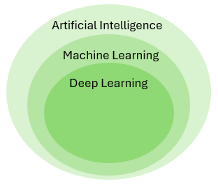
This section provides a conceptual, high-level introduction to how deep learning models for image segmentation work. Deep learning models are a subgroup of machine learning models. In broad terms, they are mathematical models that learn patterns directly from data. What distinguishes deep learning from other machine learning approaches is the use of neural networks-model architectures originally inspired by the way biological neurons are organized (hence the name).
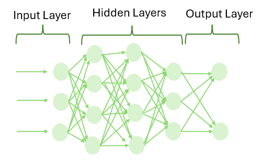
A neural network consists of a set of interconnected neurons arranged in layers: an input layer, one or more hidden layers, and an output layer. The term deep refers to the use of multiple hidden layers, which allows the model to learn increasingly complex patterns in the input data.
There are many different types of deep learning models, designed for different problem domains. Examples include large language models (such as ChatGPT) and image-based models for tasks such as classification. In the context of Visiopharm, deep learning is used for image segmentation and classification in medical image analysis. The models employed by Visiopharm are semantic segmentation models designed specifically for medical image analysis, and it is therefore these types of models that are conceptually explained in this section.
Basic Deep Learning Pipeline
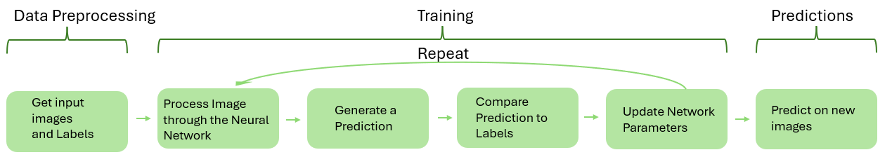
The deep learning moddeled ulitised in Visipharm are supervised moddels meaning they require labeledd data, telling them what certain objects look like, which they are then trained on in order to learn patterns.The training is an itterative process that continues undtil the moddel has learned enough from the labeled data to produces satisfactory predictions.
-
Get input images and Labels The first step in the popeline is to "get" some data for the deep learning model to train on. e.g. if the objective is to create a Deep learning app that can correctly classify tumor from stroma in lung tissue, the input data to the model should idealy be severeal lung tumor image slices, that accurate represent the tissues "you" want to analyse. These training images are then labeled such that all pixels in the image are ewither labeled as tumor or stroma. (For detailed description on how this is done see getting started).
-
Process the images through the neural network The next step in the pipeline is to compense training by feeding the training images (not the labels) through the neural network, the network then uses the network parameters also called weights to exstract features from the images, (features such as edges, color intensitives and other caracteristicas that distringush the objects in the image.) in the begining these weights are "random" but as training progresses the weights gets updated based on the prediction results to exstract more and more relevatn features and patterns frm the image. more detail on how the images are processed through the network is network arcitecture dependant and is thereofre detaile din the network arcitectures sections.
-
Generate a prediction Based on the estracted probability, the model then assigns a probability fir each class (tumor stroma e.g) for each pixel in the image, and selects the class with the higest probability as its prediction, it is this preocedure of prediction on each pixel that makes the model a semantic image segmentation model (?).
-
Compare prediction to the labels The predicted output is then compared to the drawn labels. The difference between the prediction and the correct label is used to measure how well the model is performing. this performance measure is quantified through the loss curve that measures the loss ( high is the moddel has classified a low of pixels wrong) as a function of the training iterations.
-
Update the model weights Based on the difference betwen prediction and label, the internal parameters (weights) of the neural network are adjusted to reduce the error.
-
Repeat the process Steps 2-5 are ideally repeated for many images and over multiple training iterations. Over time, the model gradually improves its predictions, as it learns from the data and adjust the internal parameters of the neural network accordingly.
-
Predict on new images Once training is complete, the trained model can be applied to new images. the model will make a prediction on the new image, (what is stroma what is tomour) based on the features and patterns about tumour stromor, it has learned on the images it has beeen trained on.
Network architectures supported in Visiopharm
In order to "fully" understand how, the images are passed through the network, and the features are exstract the network acrutecture of the selected moddel "is important.
Common for all three types of deep learning models suported by vsiopharm is, that they all make use of concolutions, pooling, (adam optimiser backproagation) in their hidden layers-.
Recall that an image is made out of pixel, and each pixel has a color intensity, (e.g. for a black and white image 0 is black and 255 is white and all numbers inbetween is different intensities of gray), for the typical RGB image each pizel contains 3 numbers corresponding to the intensity of the reg, green and blue color channel respectivly.
Typically, the encoder-decoder networks contain (1) an encoder module that gradually reduces the feature maps and captures higher semantic information, and (2) a decoder module that gradually recovers the spatial information. Bu
While many different deep learning architectures ex ist for semantic segmentation, they often share com mon structural components. These include employ ing an encoder-decoder design, skip connections, and convolutional neural networks (CNNs) as feature ex tractors.
Model. Next, the model is instantiated. A stan dard model begins with an input layer, that receives a preprocessed image from the dataset. In problems similar to root segmentation, the architecture often follows an encoder-decoder structure, where the en coder progressively reduces spatial dimensions while extracting features through convolutional and pool ing layers. The decoder on the other hand restores the spatial resolution with upsampling layers. Skip connections are often applied to preserve features April 24, 2026 Figure 20: Visual pipeline of the standard deep learning pipeline Page 21 of 80 from various layers. The final layer produces a pre diction, typically an image with the same dimensions as the input image, where each pixel holds a class label. For binary segmentation, such as root vs back ground, the output has one class.
Loss Function, Backpropagation and Optimizer. Once the model produces an output, a loss function quantifies the difference between the predicted segmentation and the ground truth. During training, the model learns iteratively using backpropagation, which computes the gradient of the loss with respect to each model parameter. These gradients are then used by an optimizer to update the model weights in a direction that minimizes the loss.
Convolutional operations are the fundamental building blocks of the UNet architecture. These operations apply small, learnable filters called kernels across the input to extract local features such as edges, textures, and shapes. INSERT IMAGE
As illustrated in Figure 22 the convolution operation involves applying a kernel to a localized region of the input image. At each position, the kernel values are multiplied element wise with the corresponding input values, and the results are summed to produce a single scalar value. For example, a kernel applied over a region might compute an output such as aw11 + bw12 +cw33 +··· +kw33, which is then interested into the corresponding position of the resulting feature map. This process is repeated as the kernel moves across the input, systematically producing the complete feature map
Several key parameters influence this operation. The kernel size determines the spatial dimension of the region processed at each step. The stride defines the step size with which the kernel shifts over the input. Finally the entries of the kernel itself determine the scaler output, they are initialized randomly at the beginning of training and are learned and updated throughout the optimization process the entirties are what is otherwise refered to as weights.
Max pooling Following the ReLU activation a 2×2×2 max pooling operation with stride two is applied. Pooling operations serve to reduce the spatial dimensions of the feature maps while retaining important information. In max pooling specifically, each local region is replaced by its maximum value, effectively preserving the strongest activations while discarding less relevant ones [10].
FCN-8s
FCN standa for Fully Connected Neural Network
UNet
The UNet model is a convolutional neural network architecture developed for biomedical image segmentation. It is characterized by a symmetrical encoder-decoder structure with skip connections, forming a U-shaped layout as shown in Figure 21. This design enables the model to combine contextual understanding with spatial precision [11], making it suitable for tasks where detailed segmentation is required from limited or incomplete annotations.
The encoder compresses the input volume through a series of convolutions and downsam pling steps, allowing the model to capture increasingly abstract features. This compression, however, comes at the cost of spatial detail. To address this, the decoder path progres sively upsamples the feature maps, reconstructing the segmentation output with the help of skip connections. These skip connections transfer high-resolution features from the encoder directly into the decoder, preserving spatial information that would otherwise be lost.
DeepLabv3
include Fig 1 from paper.
In this work, we consider two types of neural networks that use spatial pyramid pooling module [18,19,20] or encoder-decoder structure [21,22] for semantic segmentation, where the former one captures rich contextual information by pooling features at different resolu tion while the latter one is able to obtain sharp object boundaries. In order to capture the contextual information at multiple scales, DeepLabv3 [23] applies several parallel atrous convolution with different rates
Spatial Pyramid Pooling, or ASPP), while PSPNet [24] performs pooling opera tions at different grid scales. Even though rich semantic information is encoded in the last feature map, detailed information related to object boundaries is missing due to the pooling or convolutions with striding operations within the network backbone