Original Image

If Original Image is selected as the input, a specific image band can be selected for the calculation.

Add New Variable - window, with input selected as Original Image

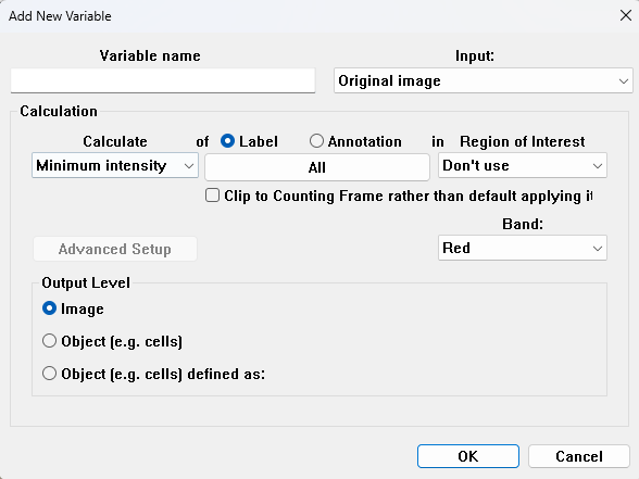
Setting	Description
Variable name	Specify a name for the variable. If the name is already in use, the variable is not added to the list.
Calculate	Select the statistical calculation to perform on the selected input. See section below for more details
Label	Specify one or all labels on which the calculation should be performed.
Region of interest (ROI)	Specify one or more ROIs to limit the calculation. Only labeled pixels within the selected ROI(s) are included. It is also possible to perform the calculation without applying any ROI restrictions.
Band	Specify the band the selected calculation should be performed (e.g., Red or HDAB - DAB).
Output level	Specifies the level at which results are reported. This setting has a significant impact on the output, determining whether a single value is generated for the entire image or individual values are generated for each object. For more information, click Output Level

warning

The interpretation of the output variable depends on both the selected calculation and the chosen output level. How results are accumulated, for instance when using the Image output level, can be found in the table Accumulation table

note

If Counting Frame is activated in the input section in the APP Control, the Counting Frame is applied on all outputs. Toggling on Clip to Counting Frame disables the Counting Frame. This is only relevant when working with larger objects that span multiple analysis tiles.

Calculate

The following calculations can be performed on the original image:

Minimum intensity

The minimum intensity of the given label or annotation for the specified feature is saved as the output variable.

Maximum intensity

The maximum intensity of the given label or annotation for the specified feature is saved as the output variable.

Mean intensity

The mean intensity of the given label or annotation for the specified feature is saved as the output variable.

Standard deviation

The standard deviation of the intensity for the given label or annotation for the specified feature is saved as the output variable.

Median

The intensity of each label/annotation is calculated in the specified frame and band. The median of the calculated intensities is saved as the variable.

Modus

The intensity of each label/annotation is calculated in the specified frame and band. The modus of the calculated intensities is saved as the variable. The modus is the most frequently occurring pixel value (if this includes several values or non-repeating values the lowest value will be saved).

Entropy

The entropy of the given label or annotation and specified band is saved as the output variable. Entropy is a measure of the randomness of the chosen chosen object, where a greater value indicates grater randomness. Entropy is estimated as a probability distribution:

$$H(X) = \sum_{i = i}^{n} P(x_i) \cdot log(P(x_i))$$

where $H(X)$ is the entropy, $n$ is the number of bins, and $P(x_i)$ is the probability of a data point falling into the $i$-th bin.

The entropy is based on a number of bins (nBins) used in the histogram calculation. Choosing many bins will allow for more precision, but will be more sensitive to noise, while fewer bins will be more resilient to noise, but might lose information.

Texture measures

The texture measurements of a given label or annotation are calculated based on the chosen band. There are six different texture measures available.

• Texture Inertia: The texture inertia is the inertia of the power spectrum. Inertia of an image can be described as the force needed to accelerate the image to a rotation around the center of the image. This means that texture inertia mainly quantifies how high the frequencies in the image are.
• Texture Entropy: The texture entropy is the entropy of the power spectrum and describes how much randomness there is present in an image.
• Texture Minor Axis: The texture minor axis is the length of the minor axis of the power spectrum, modeled as a 2-dimensional Gaussian distribution. The texture minor axis will be proportional to the frequency orthogonal to the highest frequency in the image in any direction.
• Texture Major Axis: The texture major axis is the length of the major axis of the power spectrum, modeled as a 2-dimensional Gaussian distribution. The texture major axis will be proportional to the highest frequency in the image in any direction.
• Texture Anisotropy: The texture anisotropy is the relation between the minor and the major axis of the power spectrum, modeled as a 2-dimensional Gaussian distribution. The texture anisotropy is proportional to how much directional information there is present in the image.
• Texture Major direction: This texture measurement specifies the direction of the most prominent texture. The direction is given in relation to the horizontal axis and will be between 0 and 180.

Pixel Values

The pixel value feature outputs the pixel values in a given label(s) of the given band in the current FOV (Tile analysis size). The output can create massive amount of data. The total number of included pixels in whole slides is therefore limited to the number of pixels in a single FOV.

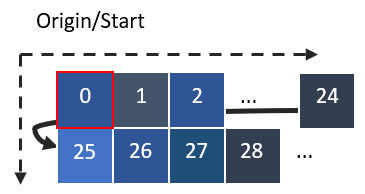
The order of the pixel data when displaying Origial Data will be as the position in the origial FOV. The first point will be the value in the top left hand corner and following values are from pixels moving left to right for each row of pixels.

Pixel Position when displaying as original data.

Unmixing

The unmixing feature provides the settings to define stain colors, automatically classify pixels to a specific stain and quantify the stain expression as an output calculation. This can be used e.g. for automatically quantifying specific protein expression inside segmented nuclei or cells in a multiplex stain procedure for IHC research applications.

Unmixing classifies the pixels to the staining/dye which they are most similar. The measure currently available is the euclidean distance in the RGB-color space defined as:

$$d \left(S^{i}_{RGB},P^{j,k}_{RGB} \right) = \sqrt{ \left(S^{i}_{R} - P^{j,k}_{R}\right)^{2} + \left(S^{i}_{G} - P^{j,k}_{G}\right)^{2} + \left(S^{i}_{B} - P^{j,k}_{B}\right)^{2} }$$

where $S^{i}$ is the $i$-th defined stain/dye and $P^{j,k}$ is the $j$-th pixel of object $k$. The similarity measure is then defined as 1 minus the normalized euclidean distance:

$$similarity \left(S^{i}_{RGB},P^{j,k}_{RGB} \right) = 1 - norm\left( d (S^{i}_{RGB},P^{j,k}_{RGB}) \right)$$

which results in 1 if the pixel is identical with the defined stain/dye.

Unmixing setup

The stains/dyes have to be defined in the Unmixing Setup, which also allows the definition of the background color which will be ignored.

The Stain Color is the real RGB color of the stain in the original image, which is defined by the user. For each selected label, a color must be chosen. To sample a color directly from the image, click the button and then click at any point on the screen. This will open a color palette to ensure that the correct color has been selected.

The Mark Option at the bottom of the dialog determines how the object or object pixels are changed in the segmentation based on the dye/stain classification:

• Do not modify object label - This will not change the segmentation result, but still output the calculation.
• Mark object with most dominating dye - This will change entire objects to the label of the dye which has the highest Mp-value.
• Mark object with most frequent dye - This will change entire objects to the label of the dye which most object pixels are closest to.
• Mark object pixels with dominating dye - This will change the objects pixels to the label of the dye which each object pixel is closest to.

Multiplexing

The multiplexing feature outputs the mean pixel band values based on the pixels included in the objects. The feature is calculated and outputted for each band in the original image. Thus, an RGB image will give a sequence of 3 numbers for each object as output, while a fluorescence image with say 5 channels will give a sequence of 5 numbers.

In the multiplexing setup, one or more color channels have to be selected, and how their pixel values contribute to the object properties. If a range for a channel is not defined, it will be ignored.

HER2IHC Connectivity

Human epidermal growth factor 2 (HER2) and Immunohistochemistry (IHC) connectivity is a measure of HER2 membranous expression with a value between 0.0 and 1.0. When selecting HER2IHC Connectivity, the gamma correction, membrane color, and object size can be edited, to provide more accurate results. Using HER2IHC requires an APP with magnication set to at least 20X, which can be set in the Input tab. To read more about the tool please refer to this HER2 Whitepaper.

Accumulation Table

The table below describes how each calculation type is evaluated depending on the selected output level. For Image as output level, a single value is calculated for the entire image. For Object defined as as output level, individual results are accumulated across the specified objects. See Output Level for more details.

Output Variable	Accumulation Type	Description
Minimum Intensity	Minimum	Keeps the lowest intensity found.
Maximum Intensity	Maximum	Keeps the highest intensity found.
Mean Intensity	Pixel-weighted mean	Calculates one average across all included pixels, so larger areas contribute proportionally more pixels.
Standard Deviation	Combined standard deviation	Calculates the standard deviation across all included pixels.
Median	Combined-histogram median	Calculates the median from the combined pixel-value distribution, respecting configured intensity limits.
Modus	Combined-histogram mode	Returns the most common pixel value from the combined pixel-value distribution.
Entropy	Combined-histogram entropy	Calculates entropy from the combined pixel-value distribution, using the configured number of bins.
Texture Inertia	Maximum	Keeps the highest texture value.
Texture Entropy	Maximum	Keeps the highest texture value.
Texture Minor Axis	Maximum	Keeps the highest texture value.
Texture Major Axis	Maximum	Keeps the highest texture value.
Texture Anisotropy	Maximum	Keeps the highest texture value.
Texture Major Direction	Maximum	Keeps the highest texture value.
Pixel Values	Append with sampling limit	Appends pixel values into an exported list. Sampling limits may cap the number retained for each field of view.
Unmixing	Element-wise sum	Adds the values for each unmixed color or label across the included objects.
Multiplexing	Count-weighted mean	Produces an average for each reported channel or band, weighted by the number of contributing values.
HER2IHC Connectivity	Stateful cumulative connectivity	Calculates connectivity cumulatively across the fields of view processed so far. It is not combined per object in the usual way.