Preproccesing Steps

A new preprocessing step can be added by clicking New Step in the define feature dialog. In this section a description of all the available preprocessing steps can be found.

Basic

Abs

By applying this step, the original pixel-value is replaced with the absolute value of the pixel. Thereby all pixel-values become positive.

Negate

By applying this step, all pixel values will be negated, resulting in black pixels turning white and white pixels turning black.

Not

By applying this step, all pixel values larger than zero are set to zero, while pixel values of zero are set to 255.

Add

This step will add either a feature image or a value to the image. To add a value, type the value in the field. To

Substract

This step will subtract either a feature image or a value from the image. To subtract a value, type the value in the field.

Multiply

This step will multiply the image with either a feature image or a value. To multiply with a value, type the value in the field.

Divide

This step will divide the image with either a feature image or a value. To divide by a value, type the value in the field.

Min

By applying this step, the input image pixels will be compared with either an input feature or a value and then choose the smallest of these.

Max

By applying this step, the input image pixels will be compared with either an input feature or a value and then choose the largest of these. This can be a useful method of combining two features.

Square

This step will square all the pixel-values of the image.

Square root

This step will take the square root of all pixel-values in the image.

Ln

This step will take the natural logarithm of all pixel values in the image.

Exp

This step will take the exponential function of all pixel values in the image.

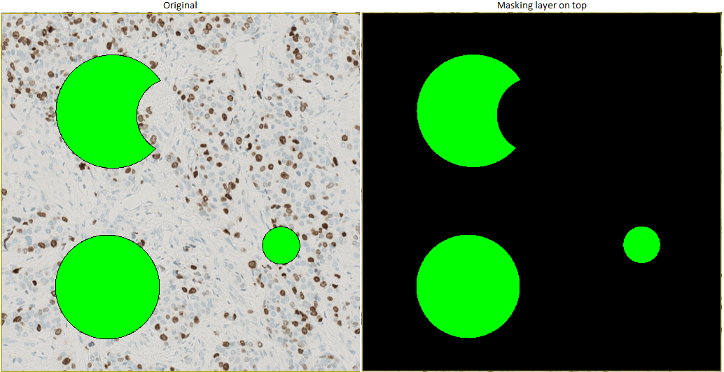
Mask

By applying this step, all pixel values outside the chosen ROI or label will be set to 0.

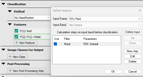
Please note that a mask step can only be applied on a feature using a separate feature as input frame.

Filters

Mean

This will run a mean-filter over the image. The idea of mean-filtering is simply to replace each pixel-value in an image with the mean ("average") value of its neighbors, including itself. The size of the filter determines how many neighboring pixels to include. This reduces noise in the image, as pixel-values which are unrepresentative of their surroundings are eliminated. The larger the filter-size the more blurred the image will become. (Note that a small filter can be applied more than once in order to produce a similar effect as a single pass with a large filter - but not identical.)

Adjusting the Temporary image size will result in a downsampling of the original image based on the percentage value. The filter is then applied over the original image and the value of the correponding pixels in the downsampled image is found using bilinear interpolation. A reduced filter is applied to the downsampled image, and the image with the filter is then sampled back to original dimensions.

Std dev

This will run a standard deviation (Std dev) filter over the image. This filter replaces the original pixel-value with the standard deviation in an area around the pixel, defined by the filter size (X- and Y-direction). Running this filter will Increase variation in the picture.

Minimum

This filter replaces the current pixel vaule with the smallest value within the area around the pixel, defined by the filter size.

Median

This will run a median-filter over the image. Like the mean filter, the median filter considers each pixel in the image in turn and looks at its nearby neighbors to decide whether or not it is representative of its surroundings. The median is calculated by first sorting all the pixel values from the surrounding neighborhood into numerical order and then replacing the pixel being considered with the middle pixel value. The filter-size determines how many neighboring pixels that are used. This process is edge-preserving, therefore the edges are not changed.

Maximum

This filter replaces the current pixel vaule with the largest value within the area around the pixel, defined by the filter size.

Modus

This will run a modus-filter over the image. A modus-filter will replace the original pixel-value with the most frequently occurring pixel-value within the area around the pixel defined by the filter size.

Polynomial Filters

Polynomial filtering is a way of approximating the image by a two-dimensional polynomial. This approximation enables the analytical computation of derivatives which are used to characterize image features such as local gradient and curvature. The order determines the largest polynomial order that can be used in this approximation. Order should always be set lower than the filter size. An order of 2-3 is often adequate.

Poly. Smoothing

This will run a Polynomial Smoothing-filter over the image. This filter is similar to a mean-filter, but the filter is bell shaped. This causes the pixels closer to the center of the filter to have a greater influence.

Poly. Gradient

This will run a Polynomial Gradient-filter over the image. The pixel-value is replaced with the value of the intensity-gradient within the filter. This is useful for edge detection.

Poly. Orientation

This will run a Polynomial Orientation-filter over the image. The filter will replace the pixel-value with the direction of the intensity-gradient within the filter. The values range between -pi and pi.

Poly. Laplace

This will run a Polynomial Laplace-filter over the image. This is a polynomial weighting of a Laplacian, which is a second derivative operator. The filter size thus determines the size of the Laplacian matrix.

Poly. Local Linear

This will run a Polynomial local linear-filter over the image. The filter is used to find elongated structures in the image. The best results are achieved with a filter of about 1.5-2 times the size of the width (in pixels) of the structures of interest. The filter enhances dark structures on a bright background, so it is important to chose an input feature that enhances the contrast between the objects to be found and the background.

Poly. Blobs

This will run a Polynomial Blobs-filter over the image. This filter will enhance round structures (blobs) in the image. Use a filter with about 1.5-2 times the same size of the diameter (in pixels) of the structures of interest. The filter enhances dark structures on a bright background, so it is important to chose an input feature that enhances the contrast between the objects to be found and the background.

Fourier Based

This will run a Fourier transformation of the image and extract the chosen feature. The spatial domain will be converted into the frequency domain - the power spectrum. The fourier based texture measurements quantifies texture by extracting different information from the power spectrum.

Four different parameters should be specified:

Filter Size

The filter size is chosen based on how many neighboring pixels that should be used.

Filter Mag

The filter magnification makes it possible to obtain a higher resolution for the Fourier transform than otherwise specified in th APP. If "As feature" is selected, the magnification will remain as specified earlier.

Step size

The step size specifies how many pixels the filter should be moved when calculating the next step. This makes it possible to optimize the processing time, i.e. while using a large filter the processing time could be minimized by applying a larger step size.

Texture

Different texture measurements are available in the dialog.

Heatmaps

This processing step will generate an Object Heatmap using a specific label and a specific object measurement. Object heatmaps can be used to visualize the intensity distribution of the slected object measurement and find hot spots.

note

This preprocessing step can only be used after a separate APP that labels certain objects has been executed.

Three different parameters should be specified:

Create Heatmap Using

Select the label that the heatmap should be based on.

Object Measure to map

Select the measurement of the selected object which the heatmap should map. Select either Object count, Object Orientation, or Object Area.

• Object Count is the number of objects withen the circle radis. I.e. when selecting the Object Count measure, the heatmap will map high density regions.

• Object Orientation is the primary orientation of the object and can be used to identify regions where objects have the same orientation. See example below.

• Object Area - Maximum, is the area of the largest of all objects within the circle radius.

• Object Area - Accumulated, is the summarized area of all objects within the circle radius.

Drawing radius

Define the raidus of the cluster circle, see below.

note

In order to find heatmap hotspots, the post-processing step Mark Max Intensity Area is used.

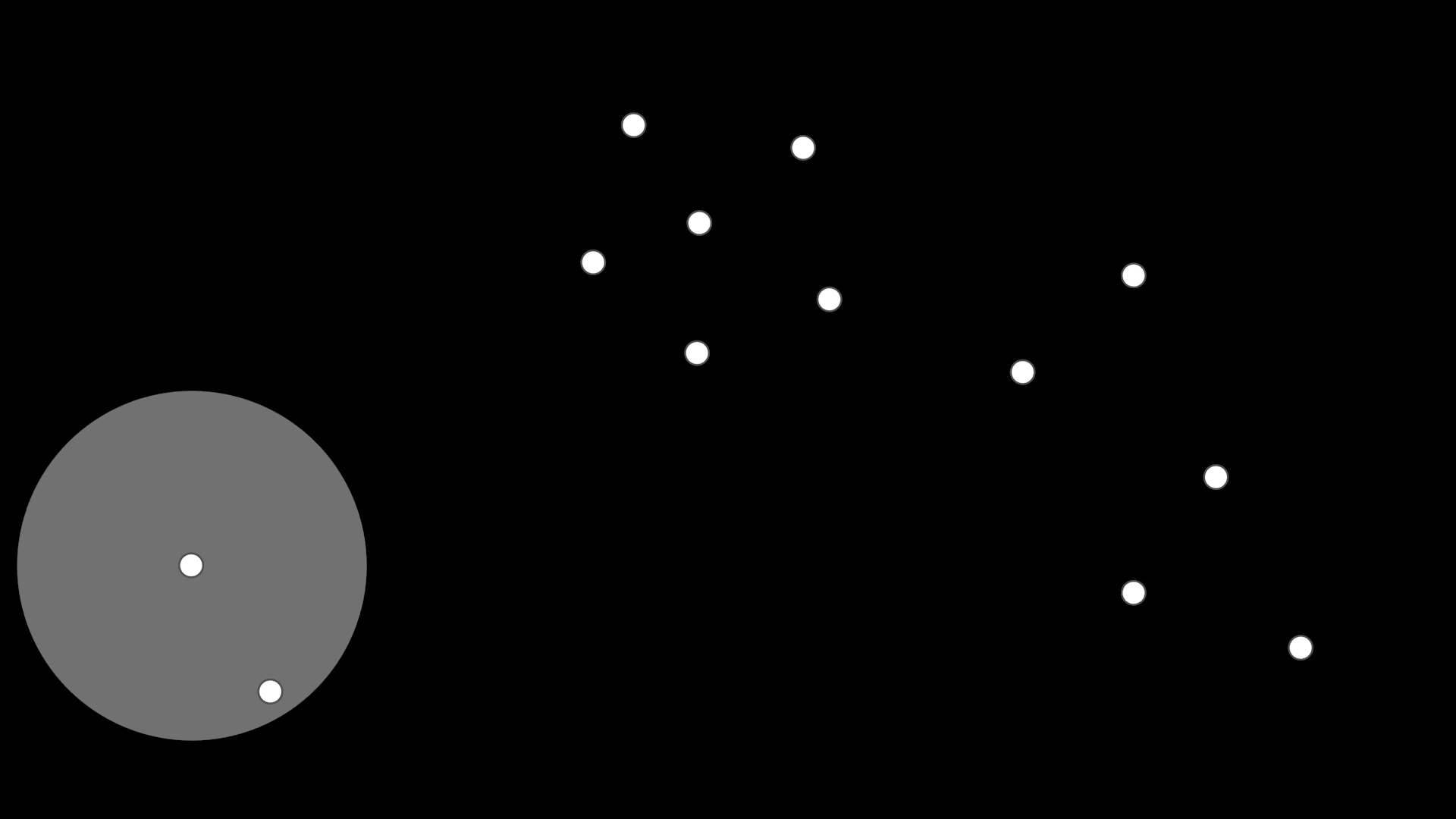
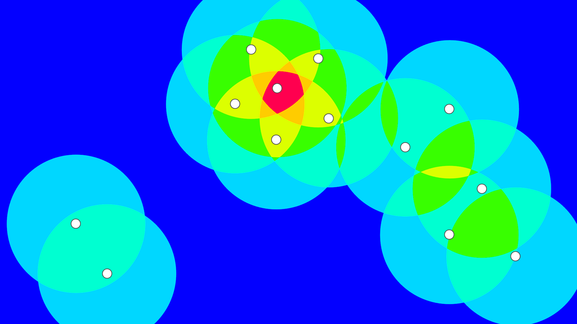
Understanding the drawing radius

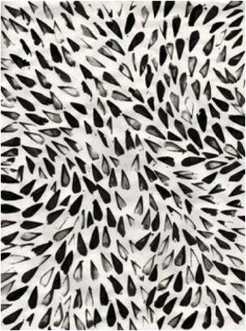
This example shows the principle of drawing radius. The images used are pseudo images which show positive cells. The selected label is positive cells and measure used is object count.

1. Define the drawing radius. In the image below, positive cells are represented by white dots while the gray circle have a radius corresponding to the drawing radius.

Cells in the 2D space with the heatmap drawing radius represented by the gray circle

2. The heatmap is generated by first creating an empty image at a much lower resolution than the virtual slide, with 0's in all pixels. If using Object Count as Object measure to map for instance, then for each label object in the image we add 1 to the heatmap image in a predefined drawing radius. The higher the radius the more blurred the heatmap will look, and the more round and cohesive the found hotspots will be.

Heatmap painted by all objects

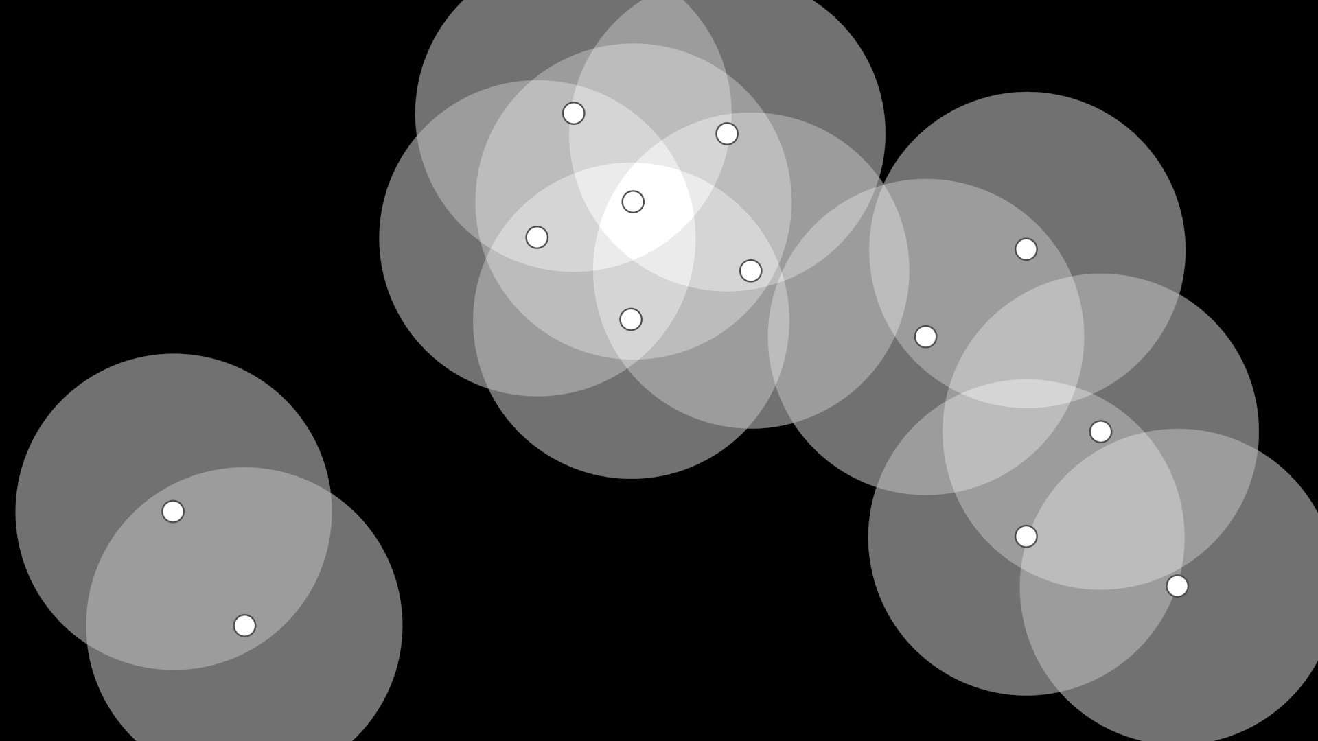
3. The heatmap is visualized using a jet colormap for providing better visual contrast compared to using a grayscale map.

Final heatmap image

Heatmap based on positive cell ratio

The heatmaps shown so far have only been based on positive nuclei. However this does not take into account cell density. A dense area might contain more nuclei, and hence more positive nuclei, and have a lower percentage of positive cells than another more sparsely populated region. Hence basing the heatmap on the ratio of positive cells may be more correct.

To create a ratio heatmap we simply create our regular positive cells heatmap and divide that by a heatmap created by looking at all cells, positive or negative. This gives us our ratio heatmap.

Note that ratio heatmaps can have tendencies to show hot spots at the periphery of the tissue: In cases where a cluster of positive cells are located at the edge of a tumor area containing a mix of positive and negative cells, the hottest area in the heatmap will be near the positive cluster, about a drawing radius away from the tumor area. The ratio will increase as the distance from the tumor area grows, as the contribution of negative cells from the tumor area will decrease accordingly.

Limit Heatmaps by conditions

In order to guide the heatmap, and subsequently where the hot spot is found, different approaches can be used.

Limit heatmap to tumor regions

If an adjacent cytokeratin slide is present, a feature can be created identifying positive tumor regions. This can then be combined with the heatmap intended for use, to display only hotspots within tumor regions.

Limit heatmap to areas with a minimum number of nuclei

Using a heatmap based on both positive and negative cells, a threshold can be set in this to indicate the minimum number of cells needed for it to be considered a hotspot. This can then be combined with the heatmap intended for use, to display only hotspots with the set minimum number of cells.

Number of cells in the hot spot

• Working with circular hot spots

  The heatmap can be limited to only show hotspots in areas with a minimum number of cells. As the area of the hot spot is fixed, the number of cells will vary depending on the tumor density, but a minimum number can be guaranteed through heatmap limiting.

• Working with heatmap shaped hot spot

  The heatmap shaped hot spot takes a minimum number of cells to include. As the hot spot follows the shape of the heatmap it will sometimes include slightly more nuclei than the minimum number, but never less.

Example of Object Heatmap

In this example, Object Heatmap is used to generate a heatmap of positive nuclei using Object Count as measure.

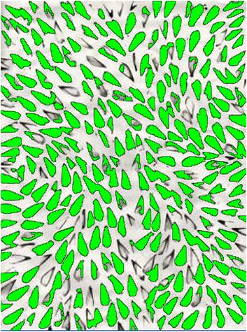
1. An APP that labels positive and negative nuclei is applied before this example with the following result:

   

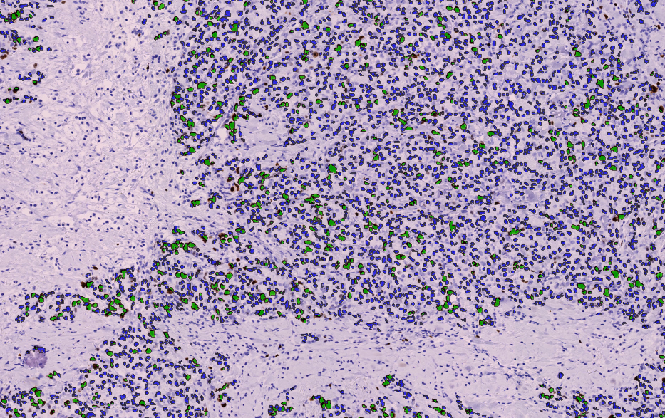
   Green labels: Positive nuclei. Blue labels: Negative nuclei (Lymph Node).

info

The Heatmap will by default, make the surrounding zero-values transparent. This behavior can be adjusted in the post-processing steps, where an option allows lower values to be made transparent. Selecting this option will render all pixels with a feature value below the minimum feature range value transparent.

2. We setup a pre-processing step that generates an Object Heatmap:

   

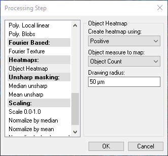
3. We then apply the processing step.

   

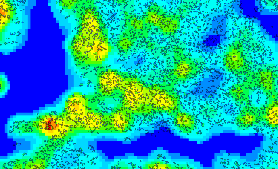
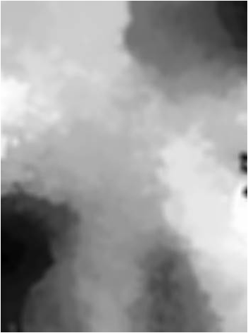
   The resulting heatmap of positive nuclei using object count. High intensity regions are red and low intensity regions are blue (Lymph Node).

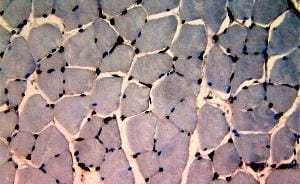
Object Measure: Object Orientation

This example shows Object Orientation as object measure.

Original image

Labeled image

Heatmap of object orientation

Unsharp Masking

Median Unsharp

This will run a Median Unsharp-filter over the image. The filter is used to remove background variation. This is done by subtracting the median within the filter from the pixel value. It is suggested to use a filter that is larger than the largest structures that need to be preserved. As with the Median-filter this process is edge-preserving, therefore the edged are not changed.

Original image (Muscle Tissue)

Red band

The red band filter after the processing step with a filter size of 25x25

Mean Unsharp

This will run a Mean Unsharp-filter over the image. This removes the background variation by subtracting the mean-value within the filter from the pixel-value. Use a filter size that is larger than the largest structures that needs to be preserved.

Scaling

Scale 0.0-1.0

This step will scale all pixel-values of the image according to the following formula:

$$NewVal = \frac{OldVal - MinVal}{MaxVal - MinVal}$$

Where the OldVal is the original pixel value, MinVal is the 1% quantile, and MaxVal is the 99% quantile. Thus pixel values less than 0 or values greater than 1 exists in the resulting band, though the majority of the pixels (98%) will be in the range of 0.0 - 1.0.

Normalize by Median

This will normalize the pixel with the median of the filter. To view the effect of this step, set Stretch in Display properties to Maximum (=x) and minimum (=y) (where the min and max values can be given). The filter is used to remove background variation. This is done by dividing the pixel-value with the median of the filter. It is suggested to use a filter that is larger than the largest structures that need to be preserved. As with the Median-filter this process is edge-preserving, i.e. the edges are not changed.

Normalize by Mean

This will normalize the pixel with the mean of the filter. To view the effect of this step, set Stretch in Display properties to Maximum (=x) and minimum (=y) (where the min and max values can be given). It removes background variation by dividing the pixel-value with the mean-value of the filter. Use a filter size that is larger than the largest structures that need to be preserved.

Normalize by Background

This preprocessing step will normalize each pixel in the FOV with the intensity of the background. It removes background variation on either light or dark background intensity by dividing or subtracting with the median of a percentage of the background image pixels.

• Background intensity - Select either Light or Dark background intensity.
• Percent of image - Enter the percentage of the image that should be used to define the background.
• Normalization type - select either Divide or Subtract.

E.g. selecting divide with 10% of the dark background intensity will normalize the image by dividing with the median of the 10% darkest pixel values.

Slide level

Scale 0.0-1.0 (WSI)

Similarly to the preprocessing step Scaling 0.0-1.0, this step will scale all pixel-values of the image between the minimum and maximum pixel values.

Scale 0.0-1.0, however, will only use the pixel values from the current Field of View, whereas Scale 0.0-1.0 (Whole Slide Image) will use pixel values from the whole image.

The check mark box allows the definition of regions of interest in the slide image, which will be the only areas considered for the scaling step (all ROIs from the whole slide). If the box is checked, the scaling will only consider pixels within the ROIs. If the box is unchecked, all pixels within the image will be considered in the processing.